Excel Workout 16 - Ifs, Sumif/s, Countif, Averageif & Round Functions!

[IlgarZarbaliyev]

Welcome to Excel Workout #16!
Difficulty Level:

This week’s challenge is designed to test your knowledge on Round, Ifs, Sumif, Sumifs, Countif and Averageif Functions.

Ifs Function
The IFS function in Excel is a logical function that allows you to test multiple conditions and return a value based on the first condition that evaluates to TRUE. It can be used as an alternative to nested IF statements and provides a more concise and readable way to handle multiple conditions.

Round Function
The ROUND function in Excel is used to round a number to a specified number of digits. It follows standard rounding rules where values equal to or greater than half are rounded up, and values less than half are rounded down.

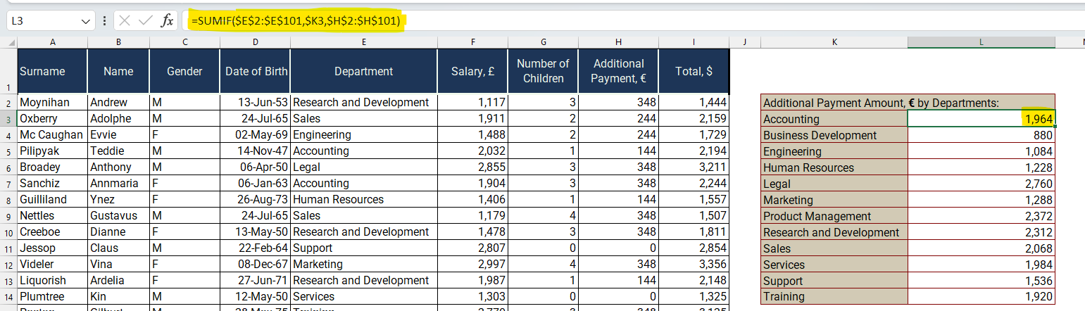
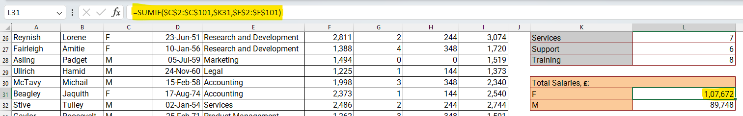
Sumif Function
The SUMIF function in Excel is used to add up values in a range based on a specified condition or criteria. It allows you to sum only the cells that meet a certain criterion, while ignoring those that do not.

Sumifs Function
The SUMIFS function in Excel is used to calculate the sum of values in a range that meet multiple criteria. It allows you to specify multiple conditions or criteria and sum only the cells that satisfy all the specified conditions.

Countif Function
The COUNTIF function in Excel is used to count the number of cells in a range that meet a specified condition or criteria. It allows you to determine how many cells in a range satisfy a certain criterion.

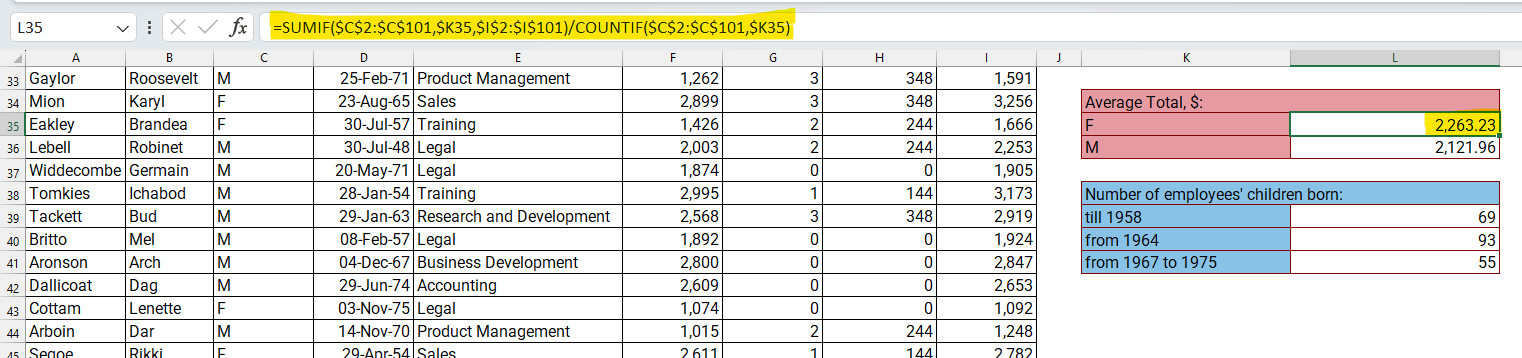
Avereageif Function
The AVERAGEIF function in Excel is used to calculate the average of values in a range that meet a specified condition or criteria. It allows you to calculate the average only for cells that satisfy a particular criterion.

Goals
Please follow the directions given below, which include downloading the Excel worksheet required to perform the challenge tasks. Once you have completed the download, proceed to take the challenge and test your skills.

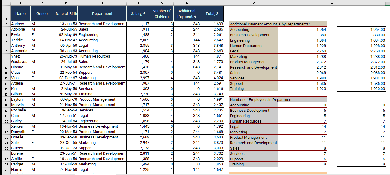
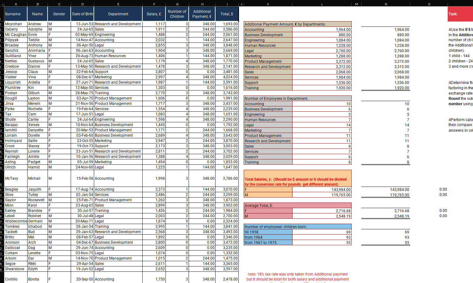
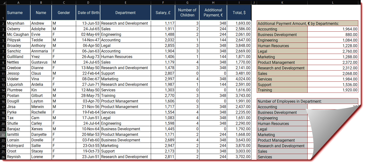
Task

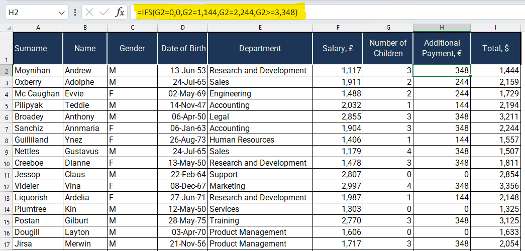
• Use the IFS function to determine the amount
  in the Additional Payment, € column by considering the
  number of children an employee has (note that
  the Additional Payment only applies to employees with
  children).
  1 child - 144
  2 children - 244
  3 and more children - 348

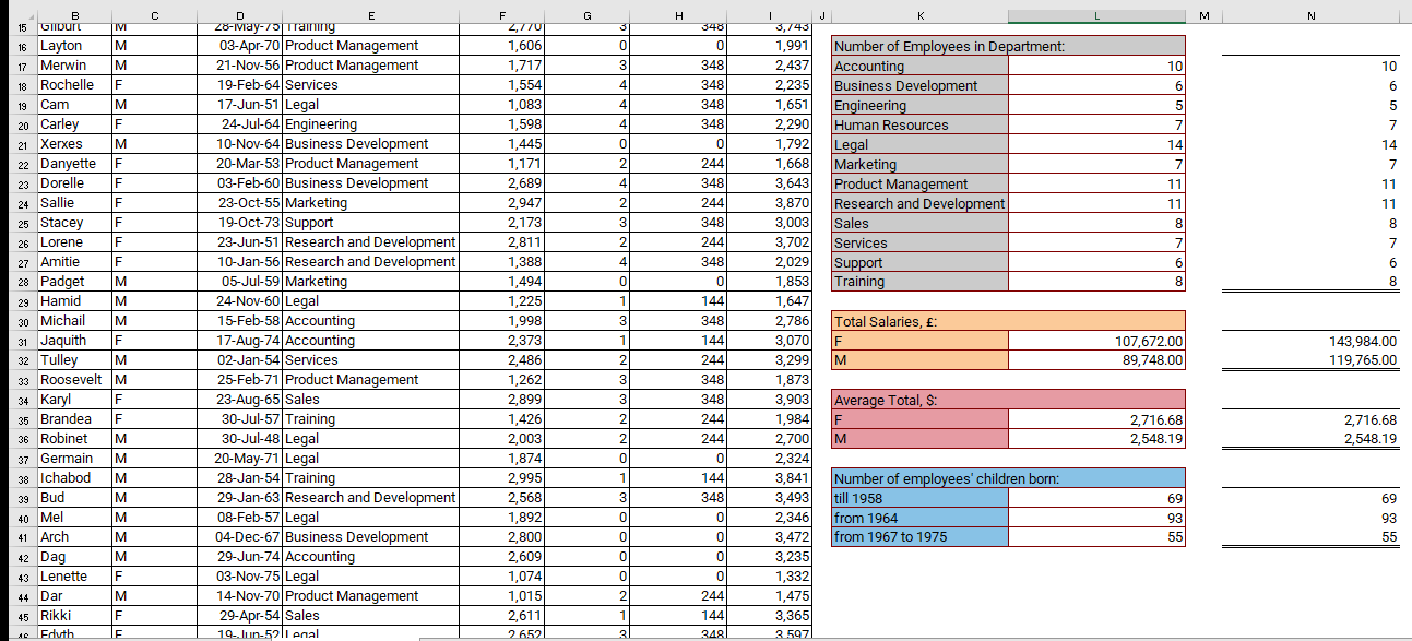
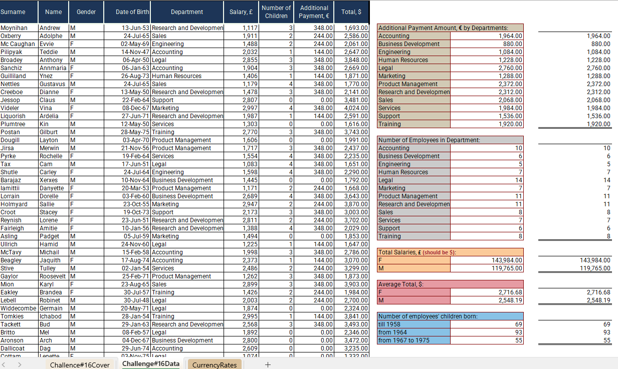
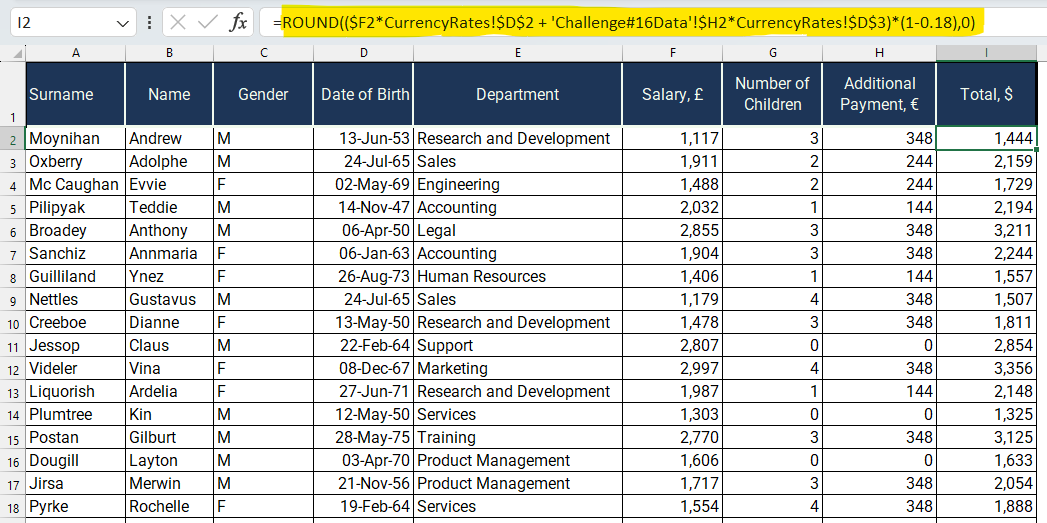
• Determine the overall sum in $ by
  factoring in the 18% tax and utilizing the
  exchange rates provided in the Currency Rates sheet.
  Round the outcome to the nearest whole
  number using mathematical principles.

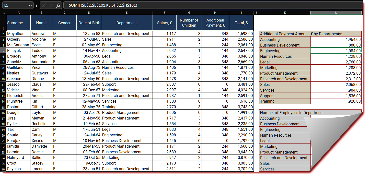
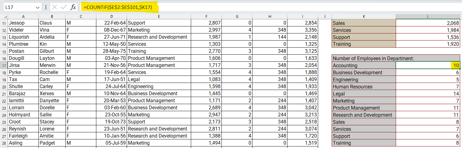
• Perform calculations on the cells within column K and
  then compare the obtained values with the corresponding
  answers in column N.

Submission
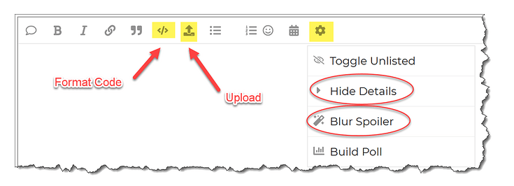
Reply to this post with your formula code and solution file. Please be sure to blur or hide your formula code.

Period
This workout will be released on Monday May 18, 2023, and the author’s solution will be posted on Sunday May 24, 2023.
Challenge #16.xlsx (8.3 MB)

Good luck,

Ilgar Zarbaliyev

[vasif_abbasov]

Challenge #16.xlsx (8.3 MB)

[BasharatAsghar]

Additional Payment:
=IFS($G2=1,144,$G2=2,244,$G2>=3,348,$G2=0,0)

Total, $
=ROUND($F2CurrencyRates!$D$2+‘Challenge#16Data’!$H2CurrencyRates!$D$3*(1-0.18),0)

Additional Payment Amount, € by Departments:
=SUMIFS($H$2:$H$101,$E$2:$E$101,$K3)

Number of Employees in Department:
=COUNTIFS($E$2:$E$101,$K17)

Total Salaries, £:
F, =SUMIFS($F$2:$F$101,$C$2:$C$101,$K31)
M, =SUMIFS($F$2:$F$101,$C$2:$C$101,$K32)

answers provided were for total salaries in $, but calculation requirement was in, £, that’s the reason both answers did not match.

Average Total, $:
F, =AVERAGEIFS($I$2:$I$101,$C$2:$C$101,$K35)
M, =AVERAGEIFS($I$2:$I$101,$C$2:$C$101,$K36)

Number of employees’ children born:
till 1958, =SUMIFS($G$2:$G$101,$D$2:$D$101,“<01/01/1958”)
from 1964, =SUMIFS($G$2:$G$101,$D$2:$D$101,“>31/12/1963”)
from 1967 to 1975, =SUMIFS($G$2:$G$101,$D$2:$D$101,“>=01/01/1967”,$D$2:$D$101,“<=31/12/1975”)

Enterprise DNA Excel Challenge #16 Solution Muhammad Basharat Asghar.xlsx (8.3 MB)

[Tural]

Additional Payment, €
=IFS(G2=1, 144, G2 = 2, 244, G2 >= 3, 348, TRUE, 0)

Total, $
=ROUND(SUM(F2*CurrencyRates!D$2, $H2*CurrencyRates!D$3*(1-0.18)),0)

To get the desired result, I had to apply 18% tax only to additional payment with this formula.

However, I personally think that tax should be applied to the total result with the following formula, which will give a different result:

=ROUND(SUM(F2*CurrencyRates!D$2, $H2*CurrencyRates!D$3)*(1-0.18),0)

Additional Payment Amount, € by Departments:

=SUMIFS(H:H,E:E,K3)

Number of Employees in Department:

=COUNTIF(E:E, K17)

Total Salaries, £ (should be $, otherwise we should convert the result which will give a different number):

=SUMIF(C:C,K31,I:I)
=SUMIF(C:C,K32,I:I)

Average Total, $:

=AVERAGEIF(C:C,K35,I:I)
=AVERAGEIF(C:C,K36,I:I)

Number of employees’ children born:

=SUMIF(D2:D101, "<01-Jan-1958", G2:G101)
=SUMIF(D2:D101, ">31-Dec-1963", G2:G101)
=SUMIFS(G2:G101, D2:D101, ">31-Dec-1966", D2:D101, "<=31-Dec-1975")

Challenge #16-TuralMammadov.xlsx (8.3 MB)

[Keith]

Hi @IlgarZarbaliyev,

Here is my solution:

Additional Payment
=IFS($G2=0,0,$G2=1,144,$G2=2,244,$G2>2,348)

Total $
=ROUND((SUM((+F2CurrencyRates!$D$2),(H2CurrencyRates!$D$3)*(1-0.18))),0)

Disagree only taking 18% out of Additional Payment should be both totals
Formula would be:
=ROUND((SUM((+F2CurrencyRates!$D$2),(H2CurrencyRates!$D$3))*(1-0.18)),0)

Additional payment amount by Department:
=SUMIFS(H:H,E:E,$K3)

Number of employees by department:
=COUNTIF(E:E,$K17)

Total Salary (should be in $ instead of british pounds)
F =SUMIFS(I:I,C:C,$K31)
M =SUMIFS(I:I,C:C,$K32)

Average Total $
F =AVERAGEIFS($I:$I,$C:$C,$K35)
M =AVERAGEIFS($I:$I,$C:$C,$K36)

Number of employees’ children born
till 1958 =SUMIF($D:$D,“<01-01-1958”,$G:$G)
from 1964 =SUMIF($D:$D,“>12-31-1963”,$G:$G)
from 1967 to 1975 =SUMIFS($G:$G,$D:$D,“>12-31-1966”,$D:$D,“<01-01-1976”)

file uploaded
Excel Workout Challenge #16 Keith Smith.xlsx (8.3 MB)

thanks
Keith

[munachimarcel]

[details="Summary"]
[spoiler]
[Munachi_Challenge #16.xlsx|attachment](upload://xWfNsh3GFkJlbZQ5nOIMwAPJS4.xlsx) (8.3 MB)

[/spoiler]
[/details]

[IlgarZarbaliyev]

Hello,
Please upload your solution once again.
Thanks in advance.

[mbraun]

So just to clear is the 18% tax on the Salary, Additional Payment or the total - unless I am missing something it is not clear by the instructions.

Also if I apply the 18% to only the Additional Payment I get the same numbers in the picture.

so if I take those # and sum them up for the M/F
Female - 143,984
Male - 119,764
This is wrong if you want it in pounds. Those are the sums of the dollar amounts.

Am I the only who is having an issue with the instructions not on how to accomplish this?

[IlgarZarbaliyev]

18% tax is deducted from the total of Salary and Additional Payment.

[ClaudiaRoxo]

Here is my file

Challenge #16.xlsx (1.7 MB)

[munachimarcel]

@IlgarZarbaliyev

18% tax is deducted from the total of Salary and Additional Payment.

this would not give the answer on the screenshot it is when 18% tax is deducted from Additional payment alone

[IlgarZarbaliyev]

I will provide the correct answer on Wednesday (25 May 2023).

[homesh_agarwal]

Table Calculations:

Calculating Additional Payment in G2:

=IFS(G2=0,0,G2=1, 144, G2=2, 244, G2>=3, 348)

Calculating Total Pay in $ in I2:

=((F2*CurrencyRates!$D$2)+('Challenge#16Data'!$H$2*CurrencyRates!D3))*0.92

Summary Tables:

• Additional Payment Amount, € by Departments:

  =SUMIF($E$2:$E$101,L3,$H$2:$H$101)

• Number of Employees in Department:

  =COUNTIF($E$2:$E$101,L17)

• Total Salaries, £- Gender-Wise
  =SUMIF($C$2:$C$101,L31,$F$2:$F$101)

• Average Total, $- Gender-wise

  =AVERAGEIF($C$2:$C$101,L35,$I$2:$I$101)

• No. of Employees born by Years: (A new column (Col J) specifying the YEAR from the Date of Birth column has been created and hidden)

  =COUNTIF(J2:J101,"<=1958")

I’ve also summarized the same data using the Pivot Tables on the right.

Challenge#16_Homesh Agarwal’.xlsx (53.3 KB)

[IlgarZarbaliyev]

Thank you for participating in the Excel Challenge related to Ifs, Sumif/s, Countif, Averageif and Round Functions! I hope you found this challenge to be a fun and engaging way to improve your Excel skills and learn more about how to work with Sumif/s, Countif, Averageif and Round Functions in Excel.

Here is my solution to Workout #16:

• Additional Payment Amount, € by Departments:
  =SUMIF($E$2:$E$101,K3,$H$2:$H$101)

• Number of Employees in Department:
  =COUNTIF($E$2:$E$101,K17)

• Total Salaries, £:
  =SUMIF($C$2:$C$101,K31,$I$2:$I$101)

• Average Total, $:
  =AVERAGEIF($C$2:$C$101,K35,$I$2:$I$101)

• Number of employees’ children born:
  =SUMIF($D$2:$D$101,“<01-01-1958”,$G$2:$G$101)
  Challenge #16 with Solution.xlsx (8.3 MB)

Once again, thank you for participating in this Excel Challenge, and I look forward to seeing you in future challenges and learning opportunities!

[Sujan_Chhetri]

Hi @IlgarZarbaliyev - please find my workout submission below:

1. Calculating “Additional Payment, €” [column H]: I have used IFs function which is an alternative to Nested IF statement.
   =IFS(G2=0,0,G2=1,144,G2=2,244,G2>=3,348)
   

   

2. For “Total, $” calculation I have deducted 18% tax from the total payment and then rounding the figure to nearest whole number. Therefore, my values are different than what @IlgarZarbaliyev had shown in his solution.
   =ROUND(($F2CurrencyRates!$D$2 + ‘Challenge#16Data’!$H2CurrencyRates!$D$3)*(1-0.18),0)
   

   

3. Additional Payment Amount, € by Departments:
   =SUMIF($E$2:$E$101,$K3,$H$2:$H$101)
   

   

4. Number of Employees in Department:
   =COUNTIF($E$2:$E$101,$K17)
   

   

5. Total Salaries, £:
   =SUMIF($C$2:$C$101,$K31,$F$2:$F$101)
   

   

6. Average Total,$:
   =SUMIF($C$2:$C$101,$K35,$I$2:$I$101)/COUNTIF($C$2:$C$101,$K35)
   

   

7. Number of Employees’s children born till 1958:
   =SUMIF($D$2:$D$101,“<01-01-1958”,$G$2:$G$101)

8. From 1964: =SUMIF($D$2:$D$101,“>31-12-1963”,$G$2:$G$101)

9. From 1967 to 1975 : =SUMIFS($G$2:$G$101,$D$2:$D$101,“>31-12-1966”,$D$2:$D$101,“<01-01-1976”)

My workout Excel File:
Excel Workout 16 - Ifs, Sumifs, Countif, Averageif & Round Functions!.xlsx (8.3 MB)

[chidinmaamara.eke73]

Challenge #16.xlsx (8.3 MB)

Summary

Formula for Additional Payment = =IFS(G2=0, 0, G2=1, 144, G2=2, 244, G2>=3, 348)

Formula for Total Salary = =ROUND(SUM(F21.24,H21.08)*(1-0.18), 0)

Formula for Additional Payment Amounts by Department = =SUMIFS(Table1[Additional Payment, €],Table1[Department],E7)

Formula for Number of Employees in Department = =COUNTIF(Table1[Department],K17)

Formula for total salaries $ = =SUMIF(Table1[Gender],K31,Table1[Total Salary $])

Formula for Average Salary $ = =AVERAGEIF(Table1[Gender],K35,Table1[Total Salary $])

Formula for Employees’ Children Born = =SUMIF(Table1[Date of Birth], “<=01-Jan-58”, Table1[Number of Children])