Data validation is a feature in Microsoft Excel that allows you to control the type and format of data that users can enter into specific cells. It helps to ensure the accuracy and consistency of data by limiting the range of values that can be entered into a cell.
Conditional formatting is a feature in Microsoft Excel that allows you to format cells based on specific conditions or criteria. This means that you can apply formatting such as color, font, or borders to cells automatically based on the contents of the cell.
Goals
Please follow the directions given below, which include downloading the Excel worksheet required to perform the challenge tasks. Once you have completed the download, proceed to take the challenge and test your skills.
Task
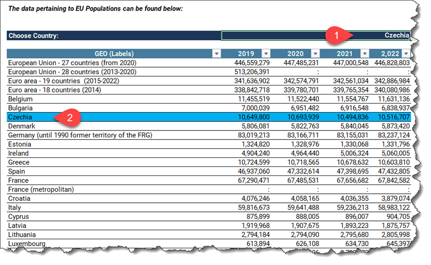
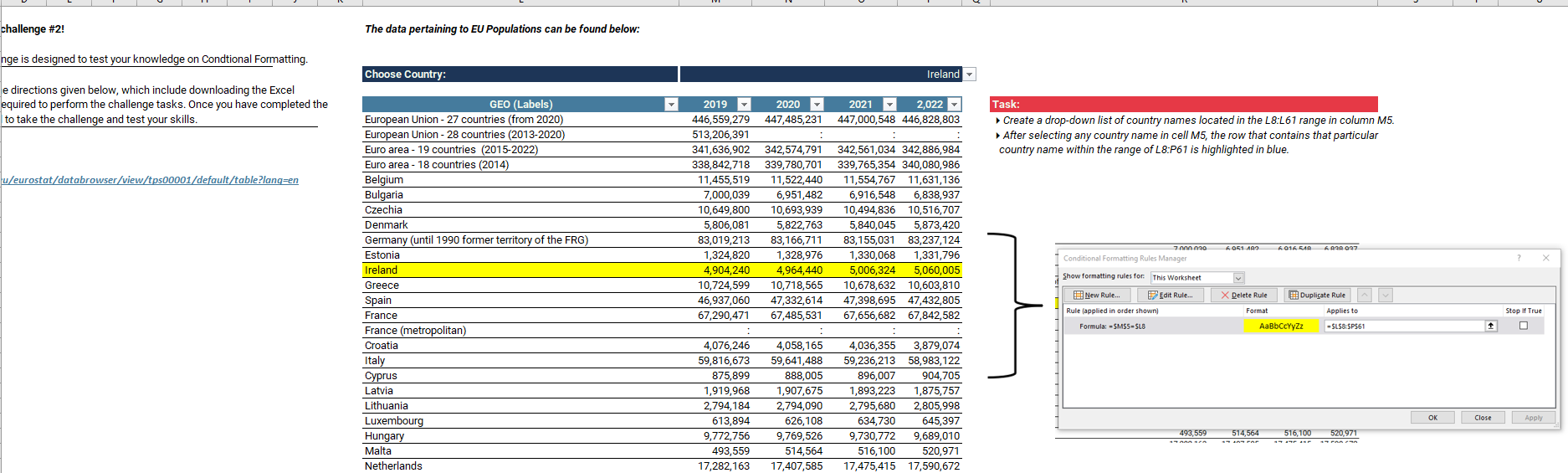
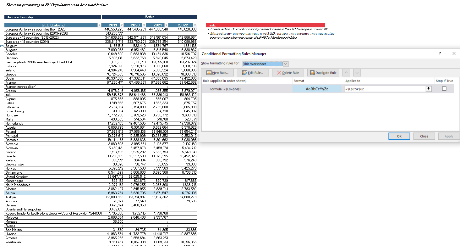
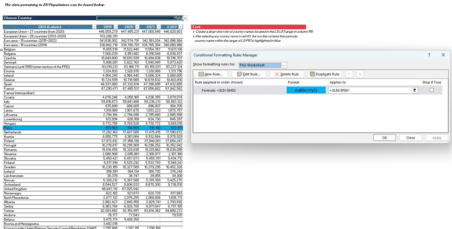
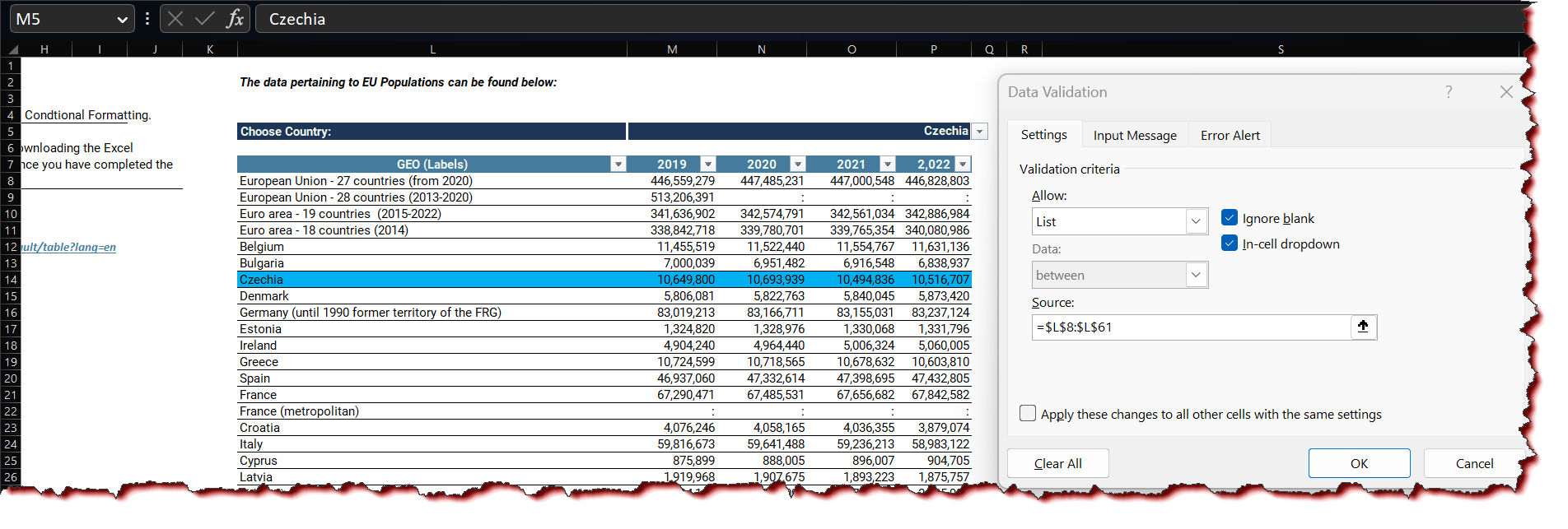
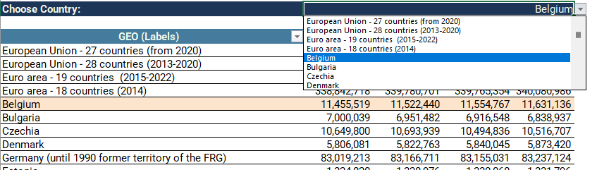
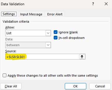
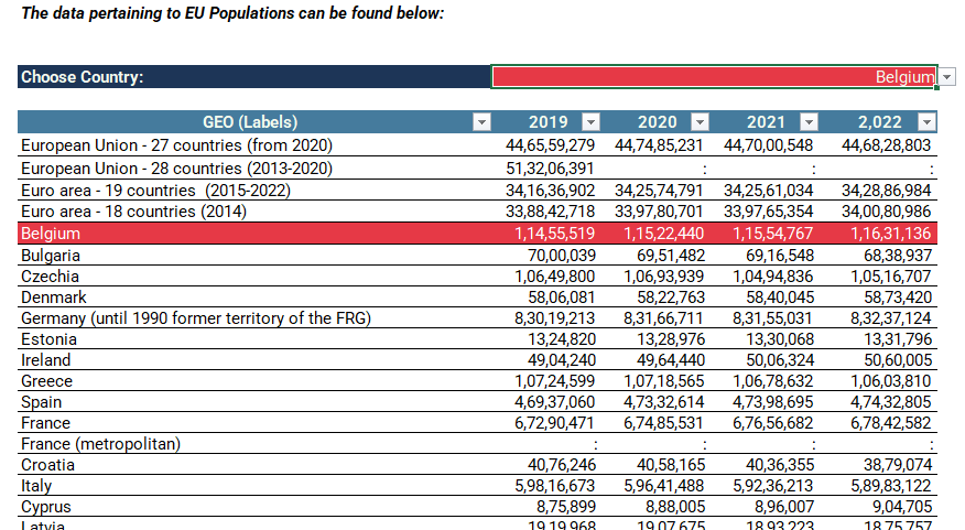
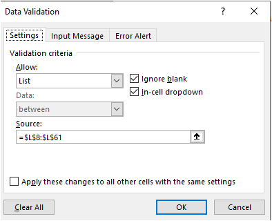
Create a drop-down list of country names located in the L8:L61 range in column M5.
After selecting any country name in cell M5, the row that contains that particular country name within the range of L8:P61 is highlighted in blue.
Submission
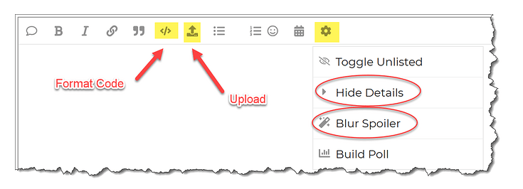
Reply to this post with your formula code and solution file. Please be sure to blur or hide your formula code.
Thank you for participating in the Excel Challenge related to Data Validation & Conditional Formatting! I hope you found this challenge to be a fun and engaging way to improve your Excel skills and learn more about how to perform conditional summation in Excel.
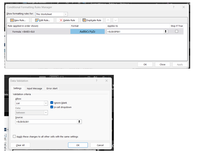
Click on Data Tab, select Data Validation from Data Validation.
Select L8:P61 Range.
Conditional Formatting
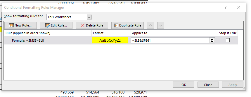
Go to Styles Group from Home Tab and click on Conditional Formatting.
Click on New Rule.
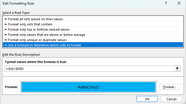
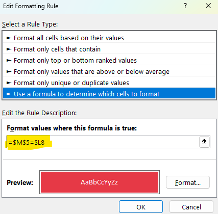
Select Use a Formula to detect which cells to format
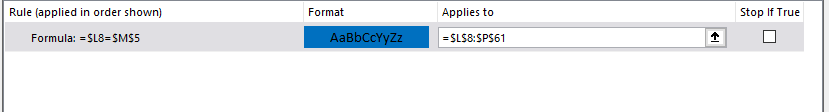
Enter the following formula in the textbox of Format values where this formula is true: $L8=$M$5
lick on Format. Select Fill Tab. Select Blue color.
Click OK.
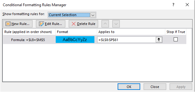
Hint: If you plan to highlight all the row based on the criteria from drop-down list, your formula that you are going to use in Conditional Formatting must be referenced.
It our case, L column has been referenced with $ sign.