Excel Workout 13 - Vlookup & Left Functions!

Welcome to Excel Workout #13!
Difficulty Level:

image

This week’s challenge is designed to test your knowledge on Vlookup & Left Functions.

Vlookup Function
The VLOOKUP function in Excel is a powerful tool for searching and retrieving data from a table. VLOOKUP stands for “Vertical Lookup,” which means that it searches for a value in the first column of a table and returns a corresponding value from a specified column in the same row.

Left Function
The LEFT function in Excel is a built-in text function that allows you to extract a specified number of characters from the beginning of a text string.

Goals
Please follow the directions given below, which include downloading the Excel worksheet required to perform the challenge tasks. Once you have completed the download, proceed to take the challenge and test your skills.

Task

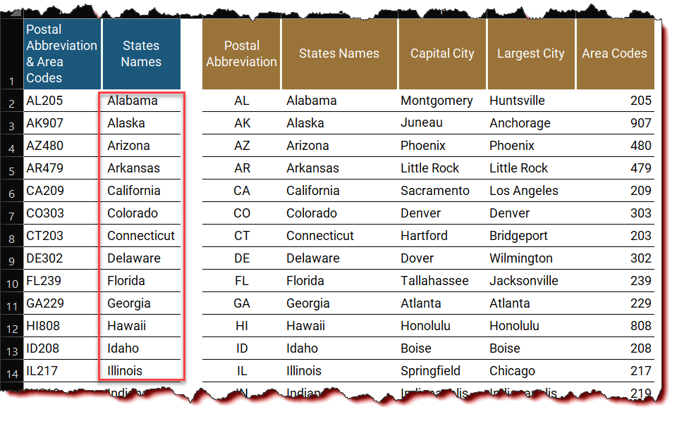
  • Based on the Postal Abbreviations and Area Codes of the
    States in the range A2:A51, type the names of the
    corresponding states in the range B2:B51

Submission
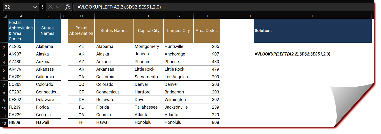
Reply to this post with your formula code and solution file. Please be sure to blur or hide your formula code.

Period
This workout will be released on Monday May 08, 2023 , and the author’s solution will be posted on Sunday May 14, 2023 .

Challenge #13.xlsx (8.3 MB)

Good luck,

Ilgar Zarbaliyev

`Seeing that the Area codes and the Postal Abbreviation are unique, we can use either to check or use the two.

`USING POSTAL CODE ABBREVIATION ONLY AS THE LOOKUP RANGE
One cell result- This will require dragging down.

> =VLOOKUP(LEFT(D2,2),$D$2:$E$51,MATCH($B$1,$D$1:$E$1,0),0)
`
.

Match is used here to ensure no hardcoding of formulas.

USING POSTAL CODE ABBREVIATION ONLY AS THE LOOKUP RANGE
For Spilled result for the whole of the postal abbreviations as below.


=VLOOKUP(LEFT(D2:D51,LEN(D2:D51)),D2:E51,MATCH(B1,D1:E1,0),0)

or
=VLOOKUP(LEFT(D2:D51,2),D2:E51,MATCH(B1,D1:E1,0),0)

USING POSTAL CODE ABBREVIATION AND AREA CODES AS THE LOOKUP RANGE
=VLOOKUP(A2:A51,CHOOSE({1,2},D2:D51&H2:H51,E2:E51),2,0)

We can decide to hardcode the length of the abbreviation by 2. or use the LEN function. Both will still work fine considering the fact that it’s uniform.
For the second and third alternatives it will not also require absolute referencing.
`
I decided to stick to old formulas and not used any of the new formulas…

Challenge #13 - Quadri VLOOKUP.xlsx (8.3 MB)

1 Like

Hi @IlgarZarbaliyev,

thanks for the workout. Its a good review.

I did it two ways:

=VLOOKUP(LEFT(A2,2),D:E,2,FALSE)
=VLOOKUP(LEFT(A2,2),$D$2:$E$51,MATCH($B$1,$D$1:$E$1,0),0)

Summary

This text will be hidden

File attached

Excel Workout Challenge #13 Keith Smith.xlsx (8.3 MB)

Thanks to the workout
Keith

1 Like

Nice to do a little excel exercise after a while working in PBI :slight_smile:

=VLOOKUP(LEFT($A2,2),$D$1:$E$51,2,FALSE)

Hannah Oldroyd_Challenge #13.xlsx (8.3 MB)

1 Like

Thank you for your solution, @HannahOldroyd.

I strongly believe that you will also participate in next challenges…
Good luck from now.

Here is my file.

Challenge #13.xlsx (1.7 MB)

1 Like
=VLOOKUP($D2,$D$2:$H$51,2,FALSE)
[Munachi_Challenge #13.xlsx|attachment](upload://vjV8Hbz1pbcv1clLE1iOYS1wovx.xlsx) (8.3 MB)

1 Like

Hi @IlgarZarbaliyev

Thanks. My attempt attached.
Challenge #13.xlsx (8.3 MB)

1 Like

Thank you for participating in the Excel Challenge related to Vlookup & Left Functions related Workout! I hope you found this challenge to be a fun and engaging way to improve your Excel skills and learn more about how to work with Vlookup & Left Functions in Excel.

Here is my solution to Workout #13:

Challenge #13 with Solution.xlsx (8.3 MB)

Once again, thank you for participating in this Excel Challenge, and I look forward to seeing you in future challenges and learning opportunities!

Hi @IlgarZarbaliyev it was a nice workout. Looking forward to solve more challenges.

[spoiler]This text will be blurred[/=VLOOKUP(LEFT(A2,2),D1:H51,MATCH(B1,D1:H1,0),0)]
Challenge #13 Golam Mohammad Sardar.xlsx (8.3 MB)

1 Like

Here’s my solution

=VLOOKUP(LEFT(A1,2), D:E, 2, FALSE)

Reliving my excel days!

1 Like

Hello @Sam,
Thank you for your answer.
I look forward to receiving your solutions for next challenges.

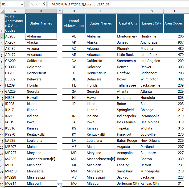
Formula to get the States Names: I have given a name to the range $D$1:$H$51 as “Location” and used the same in the formula. =VLOOKUP(LEFT($A2,2),Location,2,FALSE).

Sanpshot of the solution:


Here’s my workout file: Challenge #13.xlsx (8.3 MB)

1 Like

Challenge #13.xlsx (8.3 MB)

Summary

This text will be hidden

1 Like

I look forward receiving other solutions:)

i’ve got one, since we are looking vertically =IF(D2&H2=A2,E2,“”)