If you haven’t been living under a rock then you must be aware of Context transition, one of the most complex topics to understand and master but have you ever wondered, what actually happens behind the scenes? To be honest at least for me the behind the scene stuff is much more clear and easy to understand.
Without diving too deep into theoretical aspect, If I have to explain context transition to a layman I had say take every value of all the columns of the current row in which a measure or an expression inside CALCULATE is called and then convert all the row values into a filter context under which the measure will be evaluated. And this is done for each row of the table where measure is called.
And behind the scenes Context Transition it is just like a VLOOKUP between two data cache.
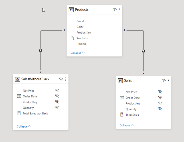
Snapshot of the data model (Contoso) used:
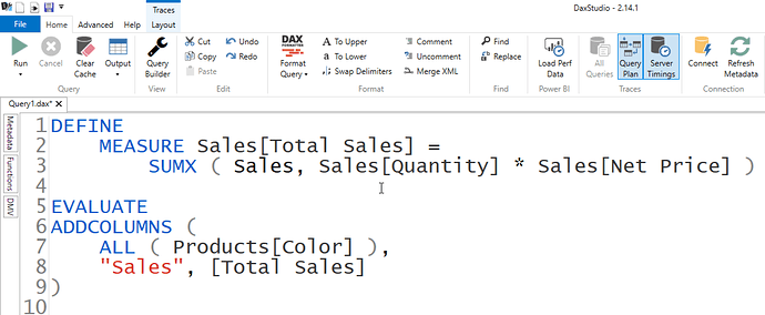
If you connect your model to DAX Studio and turn on Query Plan and Server Timings and run a simple query like the one below:
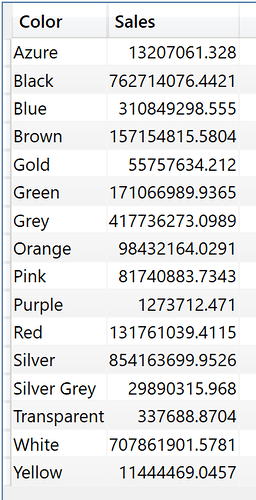
The result you get is list of unique products with the sale amount:
Now if you navigate to the server timings tab you will see 2 xmSQL ( pseudo SQL code, converted from binary to text for interpretation by humans ) queries.
The first Vertipaq query returns a data cache that has a list of Products[Color] and Sales Amount, the #Rows is just an estimate and in reality data cache only has 16 rows which is visible in the Physical query plan.
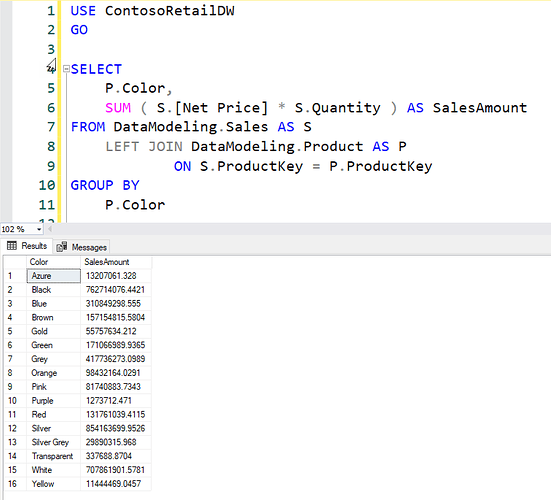
SQL equivalent of the above xmSQL code is:
Notice xmSQL has no GROUP BY but SQL has and still results are the same! that’s because xmSQL does grouping automatically whenever you select a column.
The second Vertipaq query returns a data cache containing list of Distinct Products[Color], and in xmSQL columns are always grouped automatically so there is no need to write SQL equivalent which is
SELECT DISTINCT Products[Color] FROM DataModeling.Products
The first question that comes to mind is why is there a need to get a distinct list of products color in the second Vertipaq query when the result is already obtained in the first xmSQL Storage Engine query? The reason is xmSQL puts Sales table on the LEFT side and Products table on the RIGHT side and only those rows that exists in the Sales table with a matching color are returned, in a scenario where you want to get the colors for which there is no sales you need to put Products table on LEFT and Sales table on the RIGHT side, but that’s not allowed as we can’t manipulate xmSQL directly.
These 2 data caches are used later by Formula Engine to do a lookup between data cache containing Products[Color] and other data cache containing Products[Color] and [Sales].
Remember Formula Engine can’t directly interact with the data compressed by Storage Engine, therefore it needs uncompressed data cache by Storage Engine which is materialized and then stored in memory for use later by Formula Engine, size of both data cache in this example is 1 KB.
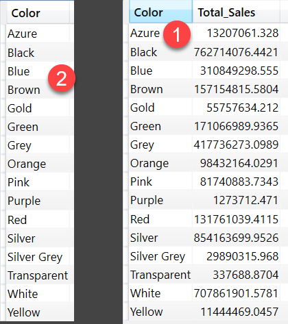
The two data cache internally will look like the below image: FE Engine will iterate second data cache and will retrieve values from the first data cache, the process is more evident in the Physical Query Plan.
==================================================================================
==================================================================================
Logical Query Plan:
The First operation is AddColumns:
RelLogOp means Relational Logical Operator which returns a table of rows and columns
DependOnCols means if ADDCOLUMNS is dependent on any outer column but in this case it is not so it has empty brackets, RequiredCols means the columns required by ADDCOLUMNS to perform the task
(Internally Formula Engine creates a Tree of objects involved in a DAX Query Plan, objects on Right side of the Tree depend on the objects on the Left Side of the Tree, in this case Products[Color] is on the left side, and extension column Sales is on the Right side of the tree, that’s why [Total Sales] measure depends on Products[Color] for its value)
The next step is to do a Scan of Vertipaq which returns the data cache #2 containing DISTINCT Products[Color] this again doesn’t depend on anything, but requires Products[Color]
Next Step is to get the Sales Amount for which the whole operation is executed inside Vertipaq SE, by operation named Sum_Vertipaq, and it has ScaLogOp (Scalar Logical Operator) property which means it returns a single value, which depends on the Products[Color] on left side of the Data Structure Tree or in simple words the first argument of ADDCOLUMNS and the type of data returned is Currency. So for each row of Products[Color] you are getting Sales Amount
For summing values inside Vertipaq, First there is a scan of Vertipaq which scans Vertipaq for 3 columns i.e. Products[Color], Sales[Quantity], Sales[Net Price]
Next Sales[Quantity] and Sales[Net Price] are multiplied to get Sales Amount
==================================================================================
==================================================================================
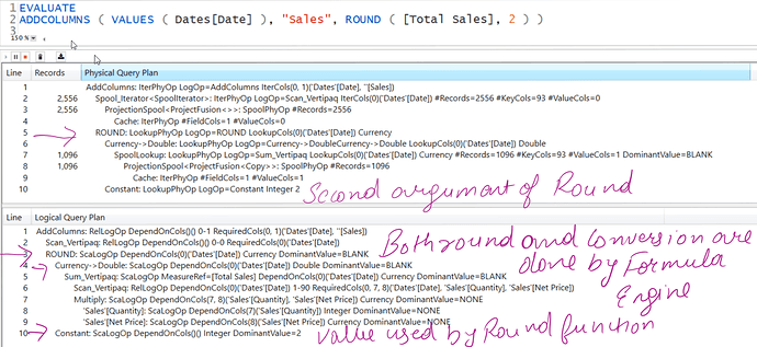
Physical Query Plan is fairly simple yet difficult in appearance:
First Step is AddColumns, The equivalent Logical Plan operation is AddColumns, IterCols means the columns returned by this operation, i.e Products[Color] and [Sales]
From Line 2-4 and 5-7 you have two Spool operations, Spools are temporary space in memory that hold data
Spooling is a process in which data is temporarily held to be used and executed by a device, program or the system
The first Spool is of type Iterator and the second one is a Lookup spool.
#Records means the rows in the data cache, #KeyCols means the columns included in the data cache but trivial ones are compressed to 0 bit hence the overall size of data cache is 1KB, #ValueCols is the number of extension column which in this case is [Sales], notice how Line 2 and 4 have #ValueCols=0 and Line 5 and Line 7 have #ValueCols = 1
Line 3 and 4 indicates the result of second SE query which is list of distinct colors
Line 6 and 7 indicates the result of first SE query which contains 2 columns which are Products[Color] and [Sales]
The Spool_Iterator operator at Line 2 supplies data from the data cache row by row to the Spool Lookup operator and Line 5 and at this point FE does a lookup between 2 data caches
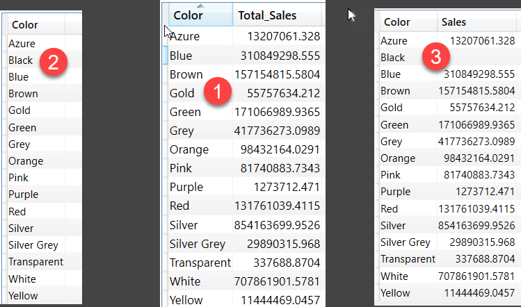
Earlier I mentioned that xmSQL puts Sales table on the LEFT side for getting Sales Amount by Product Color, but Let’s say Black color in the data model is missing Matching rows in Sales table, if DAX Formula Engine were to only use the result of the first data cache, Black would have never been included in the final result, but because Second data cache is extracted so we get to see blank for Black color after Formula engine does the lookup between 2 data cache. In the below image 1 refers to first data cache, 2 refers to second data cache, 3 is the result of lookup between 1 & 2, notice that Black isn’t in 2 but is in 1.
If xmSQL didn’t put the Sales on the LEFT side then a single SE query would have been enough to answer the original DAX query.
Contoso Sample.pbix (392.2 KB) is the sample of PBI file used, I have limited the rows to 100K due to the size of the file.
