Revenue applied over time

dsiffredi · April 7, 2020, 6:57pm

Hello , I’d like to know if someone could help me out to figure a formula to spread a new work sold figure. Say I sold $7M in January, then I want to see how revenue flows in at a specific rate which is coming from this table below. For example if I sold 7 million in January , then the revenue expected for January is as in P7 (2% jan, 9% feb, 11% march … so on and so forth).
is there an specific technique I could use to get this calculated in powerbi?
below the matrix I want to use to calculate revenue spread over time

	Jul	Aug	Sep	Oct	Nov	Dec	Jan	Feb	Mar	Apr	May	Jun
P01	2.3%	8.9%	10.6%	9.6%	9.2%	8.1%	7.6%	7.1%	6.5%	6.0%	5.8%	5.5%
P02	0%	2%	9%	11%	10%	9%	8%	8%	7%	7%	6%	6%
P03	0%	0%	2%	9%	11%	10%	9%	8%	8%	7%	7%	6%
P04	0%	0%	0%	2%	9%	11%	10%	9%	8%	8%	7%	7%
P05	0%	0%	0%	0%	2%	9%	11%	10%	9%	8%	8%	7%
P06	0%	0%	0%	0%	0%	2%	9%	11%	10%	9%	8%	8%
P07	0%	0%	0%	0%	0%	0%	2%	9%	11%	10%	9%	8%
P08	0%	0%	0%	0%	0%	0%	0%	2%	9%	11%	10%	9%
P09	0%	0%	0%	0%	0%	0%	0%	0%	2%	9%	11%	10%
P10	0%	0%	0%	0%	0%	0%	0%	0%	0%	2%	11%	10%
P11	0%	0%	0%	0%	0%	0%	0%	0%	0%	0%	2%	11%
P12	0%	0%	0%	0%	0%	0%	0%	0%	0%	0%	0%	2%

hope someone can help, I have no idea on how to tackle this one.
thanks in advance.
DanielRevenue Spread over time EnterpriseDNA.xlsx (13.2 KB)

BrianJ · April 7, 2020, 7:18pm

@dsiffredi,

I’ll give this a shot, but I’m not sure I understand the set up. Why do sales in January for example, correspond to P06? From the table, it looks like January would start with P07 at 2%, then February at 9%, March at 11% and so on.

Do you have any sample data to provide?

Thanks.

Brian

dsiffredi · April 7, 2020, 7:31pm

you are absolutely right Brian. I messed up with P6 and P7 , it should be looking P7 onwards. I’ll look for sample data I could share (as we have some data sharing restrictions here)

BrianJ · April 7, 2020, 7:44pm

@dsiffredi,

Great – thanks for the clarification. Just wanted to make sure I understood the problem properly. No big deal if you don’t have sample data. I can just randomize a quick data set - basically just sales date and sales amount, linked to a date table w/ FY starting July 1.

One more question - how do you want the output visual to look?

Thanks.

Brian

dsiffredi · April 7, 2020, 7:48pm

I’d say two ways , one format would be a table with periods and how the revenue flows in , and the other one would be a visual with either lines or bars where we can compare how new work sold is spread over time . first time I do something like this so I’m open to suggestions.
BTW: I have a very easy table I just exported with some very basic stuff. Revenue Spread over time EnterpriseDNA.xlsx (13.2 KB)

dsiffredi · April 7, 2020, 7:50pm

BTW I have a datekey table that connects Periods between sales pipeline (where the new works sold is being tracked) and the revenue conversion rates little table with the % over time.

BrianJ · April 7, 2020, 8:08pm

@dsiffredi,

Thanks – that’s really helpful. I think I’ve got the problem framed properly now. This is a really interesting one. I think it will all come down to structuring the revenue spread table in a way to make it easy for DAX to access the proper scaling factor. I’ll get cracking on this, and hopefully be back to you soon…

Brian

BrianJ · April 8, 2020, 12:41am

@dsiffredi,

OK, here goes… This one ended up being really interesting - here’s what I did:

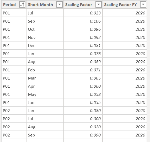
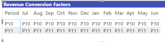
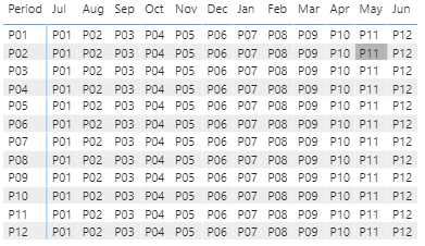
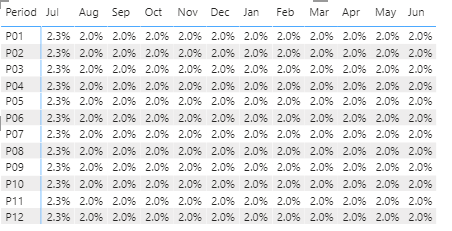
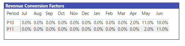
As anticipated, setting the supporting revenue scaling factor table up correctly makes it much simpler. I took your Revenue Conversion Rates Table and unpivoted all the month columns (and added a fiscal year column to make the solution more “durable” over time). Supporting table now looks like this:

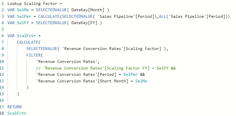
Now the measure to look up the proper scaling factor becomes a pretty straightforward CALCULATE/FILTER construct, filtering on fiscal year, period and short month:

Lookup Scaling Factor = 

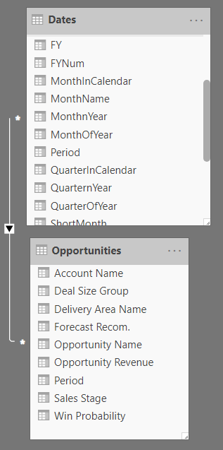
VAR SelMo = SELECTEDVALUE( Dates[ShortMonth] )
VAR SelPer = SELECTEDVALUE( Opportunities[Period] )
VAR SelFY = SELECTEDVALUE( Dates[FYNum] )

VAR ScalFctr =
    CALCULATE(
        SELECTEDVALUE( 'Revenue Conversion Rates'[Scaling Factor] ),
        FILTER(
            'Revenue Conversion Rates',
            'Revenue Conversion Rates'[Scaling Factor FY] = SelFY &&
            'Revenue Conversion Rates'[Period] = SelPer &&
            'Revenue Conversion Rates'[Short Month] = SelMo
        )
    )

RETURN
ScalFctr

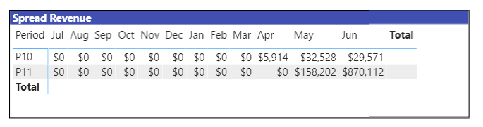
Then scaling the revenue becomes a very simple matter of multiplying revenue by the appropriate scaling factor(s):

Spread Revenue = 
[Total Opportunity Revenue]  * [Lookup Scaling Factor]

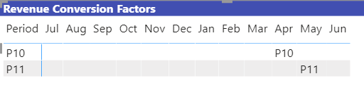
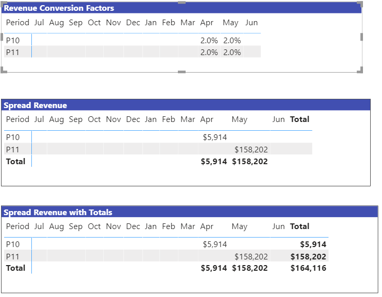
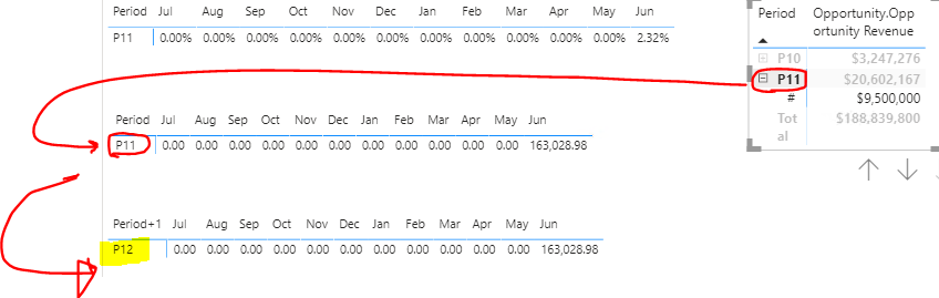
So far, so good. Just drop this measure into the matrix and…[cue sad trombone sound]

The individual cells calculate correctly, but the totals do not since they don’t have sufficient evaluation context to calculate the correct scaling factor(s). So now we have to create a measure with a virtual table of all combinations of period and short month (using CROSSJOIN) and calculate the scaling factor and scaled revenue for each row of that table. Then there are four conditions to evaluate:

both period and short month have one value - skip the virtual table and just use the measure above
short month has one value, but period does not (column totals) - SUMX of the virtual scaled revenue column over all values of period
period has one value, but short month does not (row totals) - SUMX of the virtual scaled revenue column over all values of short month
neither field has one value (grand total) - straight SUMX of virtual scaled revenue column

Here’s the measure implementing this logic:

Spread Revenue with Totals = 

VAR SelMo = SELECTEDVALUE( Dates[ShortMonth] )
VAR SelPer = SELECTEDVALUE( Opportunities[Period] )
VAR SelFY = SELECTEDVALUE( Dates[FYNum] )

VAR ScalFctr =
    CALCULATE(
        SELECTEDVALUE( 'Revenue Conversion Rates'[Scaling Factor] ),
        FILTER(
            'Revenue Conversion Rates',
            'Revenue Conversion Rates'[Scaling Factor FY] = SelFY &&
            'Revenue Conversion Rates'[Period] = SelPer &&
            'Revenue Conversion Rates'[Short Month] = SelMo
        )
    )

VAR vTable =
ADDCOLUMNS(
    CROSSJOIN(
        VALUES( Opportunities[Period] ),
        VALUES( Dates[ShortMonth] )
    ),
    "Factor", [Lookup Scaling Factor],
    "SprRev", [Spread Revenue]
)

VAR TotSpredRev = 
IF( HASONEVALUE( Opportunities[Period] ) && HASONEVALUE( Dates[ShortMonth] ),
    [Spread Revenue],
    IF( HASONEVALUE( Dates[ShortMonth] ),
         CALCULATE(
            SUMX(
                vTable,
                [SprRev]
            ),
            VALUES( Opportunities[Period] )
         ),
        IF( HASONEVALUE( Opportunities[Period] ),
            CALCULATE(
                SUMX(
                    vTable,
                    [SprRev]
                ),
                VALUES( Dates[ShortMonth] )
            ),
            SUMX(
                vTable,
                [SprRev]
            )
        )
    )
)

RETURN
TotSpredRev

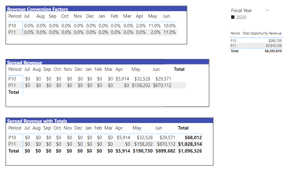
Now drop this in the matrix values well, and boom… now all totals work just as expected

Now your visuals should be easy to generate from this matrix and the above measures.

Really fun problem. Enjoyed working with you on this – hope it’s helpful. Full solution file posted below.

Brian
eDNA Forum - Revenue Spread Solution.pbix (120.7 KB)

dsiffredi · April 8, 2020, 1:12am

Brian, I wasn’t even thinking you could do that this quickly. I’ll take a look right now and see how that works on my model. I’ll let you know my findings, thank you SOOOO much for giving me such a hand .

BrianJ · April 8, 2020, 1:17am

@dsiffredi,

My pleasure. Just give a shout if you have questions or we need to tweak it for your model.

Brian

dsiffredi · April 8, 2020, 7:31am

I’ve found an issue and right now I’m stuck (12 am here so there’s the fact that I’m also tired).

the issue is that the first measure works (lookup scaling factor) IF there’s no relationship between date table and opportunities table (sales pipeline in my model) , but in my model there is a relationship and as a result when I was troubleshooting it the problem shows like this. I’m for this part rendering SelPer as the result of Lookup Scaling Value

and in reality in your example it does this.

but if you create a relationship (say for the sake of this example based on period since opportunities table doesn’t have dates just periods).

BTW: The calculated column for Opportunities table goes like this (hoping saves you time)

Period = “P” & IF(Dates[FM Number]< 10, 0 & Dates[FM Number], Dates[FM Number])

then you will see the same effect

any thoughts on how to overcome this? should I use an calculate all statement - if yes how and where. :-s
thanks again Brian. happy to do a remote session sharing desktop if this helps to troubleshoot with the live environment so we don’t go back and forth with test . I’m in US WestCoast (pacific timezone).

dsiffredi · April 8, 2020, 7:36am

I though I figured it out but something is still off.
I’ve changed this variable calculation to get the same periods accross the short months
VAR SelPer = CALCULATE(SELECTEDVALUE( ‘Sales Pipeline’[Period]),ALL(‘Sales Pipeline’[Period]))

and that seemed to work on the testing

but when calculating the final scaling factor I’ve got these weird results.
Not even close with the “original table”

BTW: We can reproduce the issue with your PBI file if we set the relationship from dates to opportunities using period

H.E.L.P

BrianJ · April 8, 2020, 1:58pm

@dsiffredi,

What should the relationship between the Date table and the Opportunities table be? The relationship isn’t needed for this calculation, since the Lookup Scaling Factor measure is basically a three-dimensional version of the LOOKUPVALUE function, which operates fine on disconnected supporting tables. But, I’d like to build our solution simulating your actual model as closely as possible.

Brian

dsiffredi · April 8, 2020, 3:11pm

good question: we use the relationship to filter dates in this case I missed to add opportunity due date in the xls file (I honestly didn’t think it will mess up anything but it did).

opportunities table is sales pipeline in the actual model.
relationship is many to one , single

BrianJ · April 8, 2020, 4:09pm

@dsiffredi,

I’m not understanding the need for DateKey. Why not just use Dates[Date] linked with Opportunity [Opportunity Due Date]? Avoids the creation of an extra key field, and Dates[Date] will validate when you mark the Dates table as a date table.

Also, can you please provide me the opportunity due dates for the sample data? Just want to be sure we are working off the same example data.

Thanks.

Brian

dsiffredi · April 8, 2020, 5:31pm

I know , I know Brian … trust me if I could get rid of that relationship I would. but the end goal is to pull data from this view and add it to backlog (another table) and datekey is key to keep things talking to eachother . I wish I could even duplicate the table, get rid of the relationship and be done. but I can’t .
I feel your frustration, I’ve been working till almost 1am my time (what I’m trying to say is that I truly appreciate your help).
attached the file updated with the due dates in it.
Also , I’ve just checked the pre-reqs and I assumed one thing wrong. when we sell say in p6 we need to apply p7 % because we won’t be getting anything that month. something I / we can work out later.
Revenue Spread Over Time EnterpriseDna.xlsx (13.2 KB)
last but not least and I’m not sure if this is the right way to do it ( so you can try this way and see if that’s the right way to do it)
I’ve used allexcept to calculate SelPer and that removed the issue when the relationship is active.
VAR SelPer = CALCULATE(SELECTEDVALUE( ‘Sales Pipeline’[Period]),ALLEXCEPT(‘Sales Pipeline’,‘Sales Pipeline’[Period]))

    Lookup Scaling Factor = 
    VAR SelMo = SELECTEDVALUE( DateKey[Month] )
    VAR SelPer = CALCULATE(SELECTEDVALUE( 'Sales Pipeline'[Period]),ALLEXCEPT('Sales Pipeline','Sales Pipeline'[Period]))
    VAR SelFY = SELECTEDVALUE( DateKey[FY] )

    VAR ScalFctr =
        CALCULATE(
            SELECTEDVALUE( 'Revenue Conversion Rates'[Scaling Factor] ),
            FILTER(
                'Revenue Conversion Rates',
                'Revenue Conversion Rates'[Scaling Factor FY] = SelFY &&
                'Revenue Conversion Rates'[Period] = SelPer &&
                'Revenue Conversion Rates'[Short Month] = SelMo
            )
        )

RETURN
ScalFctr

and to get spread revenue I have to use allexcept again to get the full table.

still learning PowerBi and this example is really tricky , thanks for your support.
here’s the relationship between backlog and pipeline (opportunities in our example)

BrianJ · April 9, 2020, 7:57am

@dsiffredi,

Had to think about this for a bit, but it turns out there’s a quick and easy workaround to the requirement of having to link the Opportunities table to the Date table. So, to make this solution work, we need a disconnected supporting table with values for Short Month, in order to do the proper lookup from the Revenue Scaling Factor table. In the initial solution I provided, I used the Date table, which worked fine until we had to impose the requirement of the relationship. However, after that relationship was created, we still have another disconnected supporting table with the same information needed for Short Month - the Fiscal Month to month supporting table I created initially to properly sort the Short Month field in the matrix header. Just do a search and replace in the measures, substituting Fiscal Month[Short Month] for Dates[Short Month], and then do the same substitution in the visuals, and it’s back to running like a champ:

Hope this gets you what you need, but give a shout if not. Full revised solution posted below.

Brian
eDNA Forum - Revenue Spread Solution2.pbix (111.5 KB)

dsiffredi · April 10, 2020, 12:02am

Simply put. YOU ARE DA MAN!!!

My god , you have no idea how difficult this thing was for me to even start thinking about . I’ll give it a try before I can call it case closed but it’s pretty darn close to be solved.

thank you so much, you won’t believe how much I’ve learned from this. how to think things thru and rethink others. Still need to figure out a few things , but trust me when I say I’m very thankful for your help.

Take care and stay safe.
Daniel

BrianJ · April 10, 2020, 3:33am

@dsiffredi,

Oh man, I know that feeling exactly. When I’ve been stuck like that, other folks on the forum have always been there to help me out, so it’s nice to be able to do the same for others. Glad that revised solution looks like it’s going to work well for you. If we need to polish it up around the edges to get it working perfectly for your particular model, just let me know.

Here’s a tip that’s worked really well for me in situations like this one - when faced with a data structure that you don’t know how to handle in Power BI, like the Revenue Scaling Factor table, think “how can I take a wide and short structure (lots of columns, few rows) and make it narrow and long (few columns, lots of rows)?” DAX handles the latter beautifully, and the former quite poorly. Once we unpivoted the scaling factor table to make it a narrow and long structure, the DAX reduced down to a pretty basic CALCULATE/FILTER structure (but for the extra rigmarole with the matrix totals). Here’s another example where “narrow and long” made life much simpler:

It won’t solve all your problems, but I’ve been surprised how often it’s the key to cracking a difficult solution.

Brian

dsiffredi · April 11, 2020, 9:17pm

good tips indeed , thanks Brian! this whole exercise taught me a lot .
I have one question, because they now want to show the results of the spread revenue on the following period.
So if something is showing as say $9 million in P11 on the opportunities table , they want apply the scaling factor of P11
BUT
they now want to see the first iteration of results on P12
why?
because is practically impossible to close any opportunity in the same month.

I honestly wish I knew this before asking you.

BTW: this is a mock up think I did adding another column to opportunity pipeline called Period+1

for example this is a $7M opty on P11 that the spread revenue should show starting in P12 (but using the scale factor for P11 of course).

sorry if this is messy …

Happy Easter if you celebrate it .
Stay safe !