Hi
In the attached workbook there are three named ranges in cells D7 G7 H7. I am going to combine multiple workbooks in a folder. Each file will have these named ranges.
When i combine the workbooks I want to be able to put each of these 3 values into a column of its own.
How do i do this?
Thank You
Allister
Book3.xlsm (12.3 KB)
Hi AlisterB,
PowerBI Steps to AlisterB:
NOTES:
-
All the Excel files should be in one folder. No other file should be there
-
All the Excel files should have data in the same places. For example, the Financial quarter number should be in column 7 for all files. If this is not the case, then the steps below will have to be modified when it comes to selecting the columns where Power BI should fetch the data from.
Please follow the instructions below:
- Click on “Transform data” to open the Query editor
- New source > More > Folder > Connect
* Select folder with the files
* Click on Transform
- Right click on the header “Content”
* Select “Remove Other Columns”
- Click on “Add column
- Click on “Custom column”
* Name it “GetExcelData”.
* In Custom Column formula type “=Excel.Workbook([Content])”. Click Ok
- Right click on the header “Content”
* Select “Remove”
- Click on the arrows on the far right of the column header “Table”
* Check / Tick “Data” i.e uncheck all except “Data”
* Uncheck “Use original name as prefix”
- Click on the arrows on the far right of the column header “Table”.
* Check / Tick Columns 4, 7,8
- Apply a filter for any column name “Column4”
- Rename Columns 4, 7 and 8 appropriately
- Rename the query appropriately
- Click on Close and Apply
Do not hesitate to ask for clarity if need be.
1 Like
Hi @AllisterB,
Will you be using this in Excel or Power BI? If it’s Excel follow these steps.
- Open the Power Query Editor
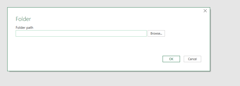
- Select “New Source”, File, Folder
- Create a “New Parameter” when prompted for the Folder path (in the drop down menu)
- Select “Combine & Transform Data”
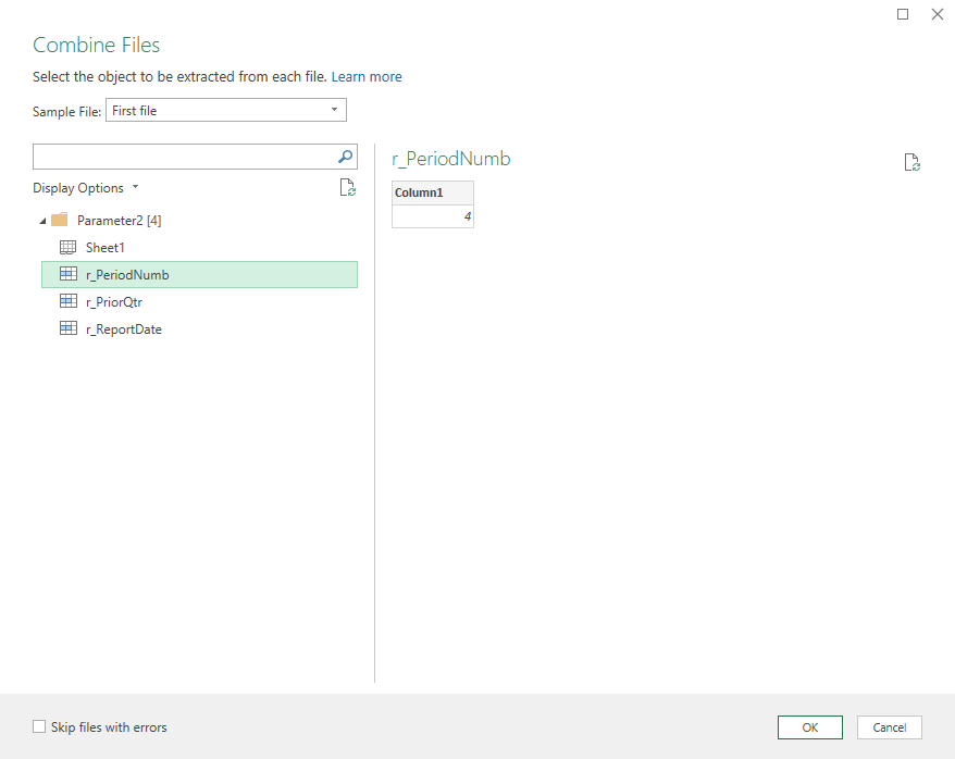
- Select one of your NamedRanges and press OK
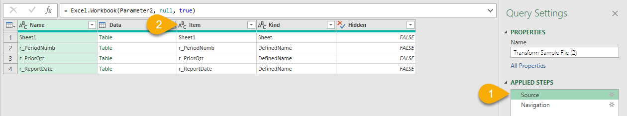
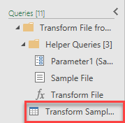
- In the Queries Pane, select the “Transform sample” query
- In the Applied Steps pane, select the Source step (and remove the second step!)
- Filter the Column “Item” starts with r_
- Remove all other columns except Name and Data
- Expand the Data Column (deselect “Use original column name as prefix”)
- On the Ribbon go to the Transform tab and select Transpose
- On the Ribbon go to the Transform tab and select Use First Row as Headers
Now in the Queries pane, select the result query and remove the Changed Type step
.
I hope this is helpful.
Thanks melissa
This looks as if it will be great
I get to step three and dont know where to go to get new parameter
This is what I have at teh end of step 2.
Thanks
Allister
Reference: @Melissa’s steps
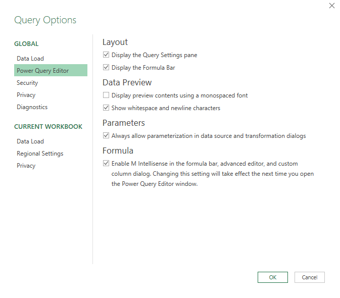
Step 3 will be automated when you select the folder that contains your Excel files. You will see the created Parameter when you get to Step 5 (See screeshot).
I believe you were on O365 right? If so, on the ribbon go to: Data, Get Data, Query Options
make sure under Parameters “Always allow prameterization…” is enabled.
Hi @AllisterB, we’ve noticed that no response has been received from you since the 19th of May. We just want to check if you still need further help with this post? In case there won’t be any activity on it in the next few days, we’ll be tagging this post as Solved. If you have a follow question or concern related to this topic, please remove the Solution tag first by clicking the three dots beside Reply and then untick the checkbox. Thanks!
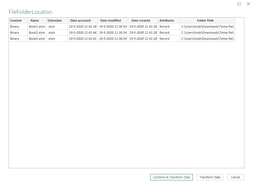
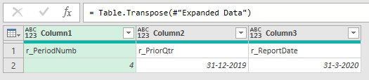
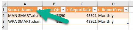
HI
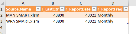
I got the the table as attached.
I am now not sure How I get these values into the combined data tablee. I have two workbooks in my folder one for MAN and one for WPA that I can combine. The attached table shows the values of the named ranges from those files. How do I now get them into three columns in my combined table.
Please note eth parameter values for MAN and WPA could be different.
I am thinking of creating three new columns, renaming to match the column names on the attached and then do a Merge ?
Allister
Which combined table?
Ps. You can change the format of the date values in the output table.
.
If your other ‘table’ is:
- created in Power Query, you could do a Merge if they share a key
- an excel worksheet range, you could use Spill functions and XLOOKUP
Hi Melissa
The combined table is the one that I get from from combine and transform. It holds the main data from the files in the folder.
Thanks
Sorry I’m still missing the point here…
Can you visualize the desired result somehow? Thanks Allister.
Hi
Looking at it a different way. If I merge the query that holds the 3 parametres with the files in the folder and use the source as the key… Will that work?
If you’re referring to this as source key, then it should if that file name is also present in the other query
Thanks for posting your question @AllisterB To receive a resolution in a timely manner please make sure that you provide all the necessary details on this thread.
Here is a potential list of additional information to include in this thread; demo pbix file, images of the entire scenario you are dealing with, a screenshot of the data model, details of how you want to visualize a result, and any other supporting links and details.
Including all of the above will likely enable a quick solution to your question.
Hi @AllisterB, a response on this post has been tagged as “Solution”. If you have a follow question or concern related to this topic, please remove the Solution tag first by clicking the three dots beside Reply and then untick the check box. Thanks!