Excel Workout 24 - Filter, Unique & Xlookup Functions (Recipe Cost Calculator)!

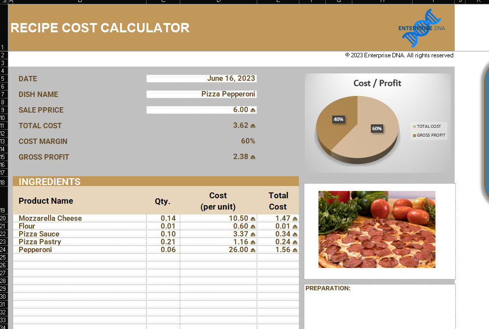
Welcome to Excel Workout #24!
Difficulty Level:

3-removebg-preview

This week’s Recipe Cost Calculator Challenge is designed to test your knowledge on XLOOKUP, UNIQUE & FILTER Functions.

XLOOKUP Function
The XLOOKUP function is a powerful lookup function introduced in Microsoft Excel 365, Excel 2021, and later versions. It is an enhanced version of the traditional VLOOKUP and HLOOKUP functions, providing more flexibility and functionality. XLOOKUP allows you to search for a value in a column or row and return a corresponding value from another column or row, with the ability to perform exact matches, approximate matches, and handle multiple criteria.

UNIQUE Function
The UNIQUE function is a dynamic array function introduced in Microsoft Excel 365, Excel 2021, and later versions. It allows you to extract unique values from a range or array of values.
The UNIQUE function automatically creates a dynamic array of unique values, removing any duplicates. This means that when you enter the UNIQUE formula into a cell, it will spill the unique values into adjacent cells automatically.

FILTER Function
The FILTER function is a dynamic array function introduced in Microsoft Excel 365, Excel 2021, and later versions. It allows you to extract a subset of data from a range based on specific criteria or conditions.
The FILTER function takes an array or range of data and returns a new array containing only the rows that meet the specified criteria. It can filter data based on one or more conditions, providing a powerful and flexible way to extract specific information from a larger dataset.
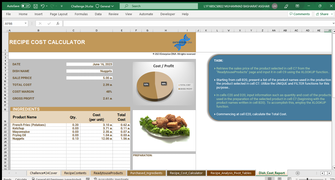
Task

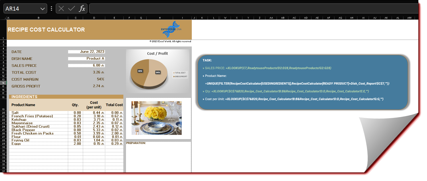
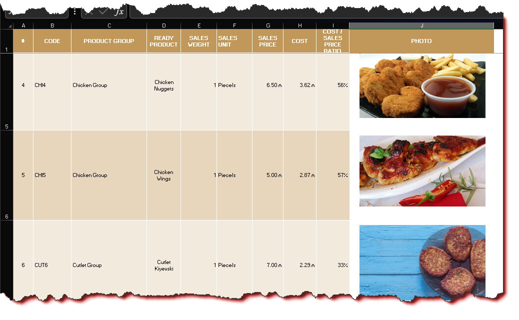
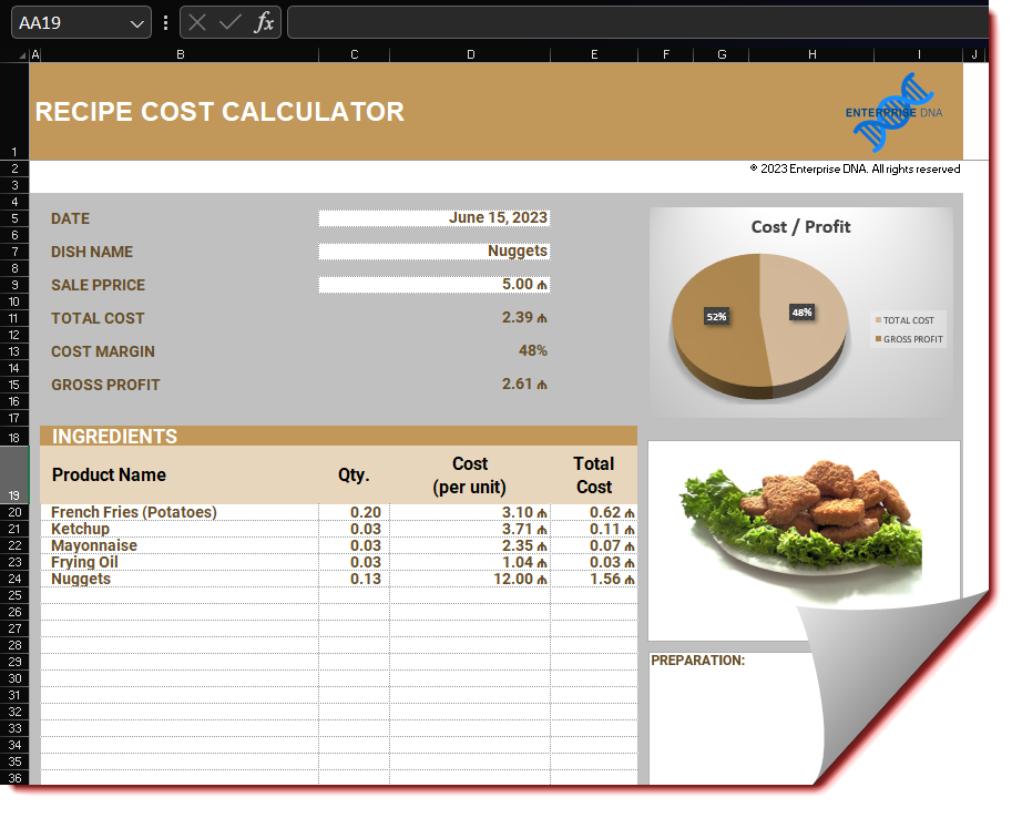
  • Retrieve the sales price of the product selected in cell C7 from the “ReadytouseProducts” page and input it in cell C9 using the XLOOKUP function.

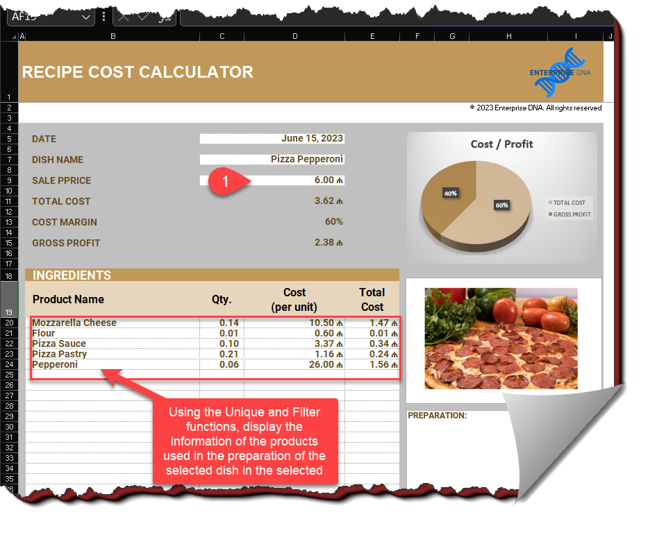
  • Starting from cell B20, present a list of the product names used in the production of the product selected in cell C7. Utilize the UNIQUE and FILTER functions for this purpose.

  • In cells C20 and D20, input information such as quantity and cost of the products used in the preparation of the selected product in cell C7 (beginning with the product names written in cell B20). To accomplish this, employ the XLOOKUP function.

  • Commencing at cell E20, calculate the Total Cost.

Submission
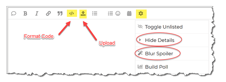
Reply to this post with your formula code and solution file. Please be sure to blur or hide your formula code.

Period
This workout will be released on Thursday June 15, 2023 , and the author’s solution will be posted on Sunday June 22, 2023.

Google Drive Link: - https://docs.google.com/spreadsheets/d/1D5e0RUYcsYkovQv-eKwzE7k0p7n2wH44/edit?usp=sharing&ouid=105695772191952708788&rtpof=true&sd=true

Download file to join the Excel Challenge 24

Good luck,

Ilgar Zarbaliyev

1 Like

Just two formulas are neccesary to do this exercise:

C9: =XLOOKUP(C7,ReadytouseProducts!D2:D28,ReadytouseProducts!G2:G28)

B20: =FILTER(CHOOSECOLS(RecipeCostCalculator,4,5,7,8),RecipeCostCalculator[READY PRODUCT]=C7)

Blessings!

1 Like

Hi @IlgarZarbaliyev,

Here is my solution to this workout. This has been a good review for me.

C9:

=XLOOKUP(C7,ReadytouseProducts!D:D,ReadytouseProducts!G:G)

B20:

=UNIQUE(FILTER(Recipe_Cost_Calculator!D:D,Recipe_Cost_Calculator!B:B=C7))

I get an error message the file is to big to upload

couldn’t load the file as the file is to big (even tried zipping the file)…please adjust your file capacity or adjust the xp points.

July 1, 2023
file uploaded after changing the picture compression. Please change the xp points
Excel Workout Challenge 24 Keith - Copy.xlsx (9.9 MB)

thanks for the workout.
Keith

1 Like

Sale Price:

=XLOOKUP($C$7,ReadytouseProducts!$D$2:$D$28,ReadytouseProducts!$G$2:$G$28)

Product Name:

=UNIQUE(FILTER(RecipeCostCalculator[USED INGREDIENTS],RecipeCostCalculator[READY PRODUCT]=C7))

1 Like

Thanks again @IlgarZarbaliyev for the challenge.
These are the formulae that I used:

`[spoiler]
``

Sales Price: =XLOOKUP(C7,ReadytouseProducts!D:D,ReadytouseProducts!G:G,“Not Available”,0)
I had to convert the table into a range otherwise the array for Product Name did not work.
Product Name: =FILTER(Recipe_Cost_Calculator!D2:D251,Recipe_Cost_Calculator!B2:B251=C7," “))
Qty: =XLOOKUP($C$7&B20,Recipe_Cost_Calculator!B:B&Recipe_Cost_Calculator!D:D,Recipe_Cost_Calculator!E:E,”“,0)
Cost Per Unit: This text will be blurred=XLOOKUP($C$7&B20,Recipe_Cost_Calculator!B:B&Recipe_Cost_Calculator!D:D,Recipe_Cost_Calculator!G:G,”“)
Total cost: =IFERROR(D20*C20,”")

I didn’t understand where to use the ‘UNIQUE’ function - so not sure if I missed something.

[/spoiler]

![image|690x381](upload://aqUGhUmeEEWL0fwsDnyFtyMNrVR.png)
1 Like

Thank you for your answer, @Abee .
I will provide my answer on Thursday.

Please paste the link

1 Like

i don’t have a link to paste @IlgarZarbaliyev

All solution files can be pasted as a link.

i can’t paste a link…i get an error when i try to paste the links…same error .( file to big)

No issue. Thank you for your solution.

Thank you for participating in the Excel Challenge related to FILTER, UNIQUE & XLOOKUP Functions (Recipe Cost Calculator)!
I hope you found this challenge to be a fun and engaging way to improve your Excel skills and learn more about how to work with FILTER, UNIQUE & XLOOKUP Functions (Recipe Cost Calculator)! in Excel.

Here is my solution to Workout #24!

Solution

  • SALES PRICE: =XLOOKUP(C7,ReadytouseProducts!D2:D28,ReadytouseProducts!G2:G28)

  • Product Name:
    =UNIQUE(FILTER(RecipeCostCalculator[USEDINGREDIENTS],RecipeCostCalculator[READY PRODUCT]=Dish_Cost_Report!$C$7,“”))

  • Qty: =XLOOKUP($C$7&B20,Recipe_Cost_Calculator!B:B&Recipe_Cost_Calculator!D:D,Recipe_Cost_Calculator!E:E,“”)

  • Cost per Unit: =XLOOKUP($C$7&B20,Recipe_Cost_Calculator!B:B&Recipe_Cost_Calculator!D:D,Recipe_Cost_Calculator!G:G,“”)

Once again, thank you for participating in this Excel Challenge, and I look forward to seeing you in future challenges and learning opportunities!

1 Like

Thank you @IlgarZarbaliyev for bringing together Challenge 24.

I thought I would share why Challenge 24.xlsx was unusually large due
to picture resolution of the images in the stored file when the file was saved.
Through the use of Excel’s CompressPictures tool, I was able to reduce the file
size from 148 MB to 1.48 MB.

Some background: Challenge 24.xlsx contained 39 images, and the file was saved with the images stored within the file using full resolution. Each of the images ranged from a few hundred kilobytes to several megabytes in size.

So, how do I determine image file size, Excel doesn’t seem to have a tool or option to do that? Easy.

Browse the Excel file as a .zip file. In other words, change the file extension from .xlsx to .zip, and then browse the zip file to the folder path ’ \xl\media\ ’ where images added to the Excel file are stored.

compress3

.

So, how do I adjust the image file size for images stored in Excel?

• File size can be reduced by changing the picture resolution by using Excel’s Compress Pictures tool (Picture Tools | Picture Format Tab | Adjust | Compress Pictures (PicturesCompress).
• Default setting can be changed in Excel Options ( Excel Options | Advanced | Image Size and Quality | Default resolution) as shown.

To save time, as I may use this often, I have pinned PictuesCompress Icon to the Quick Access Toolbar for ease of access.

A good all-rounder option is Web (150 ppi): good for web pages and
projectors, and Email ( 96 ppi) .


.
compress2
.
filesize
.
• Challenge24.xlsx before compressing all pictures in file: 147 MB (154,215,600 bytes)
• Challenge24.xlsx compressing all pictures in file (to 96ppi.): 1.48 MB (1,560,875 bytes)

1 Like

Thank you, @ystroman.
That is so great…

No prob., this is one of the day to day audit checks I still lean upon prior to publishing weekly reports . For the most part, this is a standby practice begun years ago when you had to watch attachment sizes else face the wrath of the IT.

1 Like

@IlgarZarbaliyev - Another interesting workout for me. Please find my solution below:

Formula to show Sales Price: =XLOOKUP($C$7,ReadytouseProducts!$D$2:$D$28,ReadytouseProducts!$G$2:$G$28)

Formula to display Product Name: =UNIQUE(FILTER(RecipeCostCalculator[USED INGREDIENTS],RecipeCostCalculator[READY PRODUCT]=Dish_Cost_Report!$C$7))

Formula to show corresponding Qty value: =XLOOKUP($C$7&$B20,RecipeCostCalculator[READY PRODUCT]&RecipeCostCalculator[USED INGREDIENTS],RecipeCostCalculator[USED WEIGHT],“”)

Formula to show Cost price of each Ingredient used: =XLOOKUP($C$7&$B20,RecipeCostCalculator[READY PRODUCT]&RecipeCostCalculator[USED INGREDIENTS],RecipeCostCalculator[COST],“”)

Formula to calculate total cost: =IFERROR(C20*D20,“”)

Here’s a link to my workout file: https://docs.google.com/spreadsheets/d/1_M-4oBPZnXT9gAZN2dt0W7q1W-iP2_6a/edit?usp=drive_link&ouid=115708230205732441359&rtpof=true&sd=true

1 Like

Well-done! Congrats!