R Workout 03 - Basic Time Intelligence

[KrzysztofNowak]

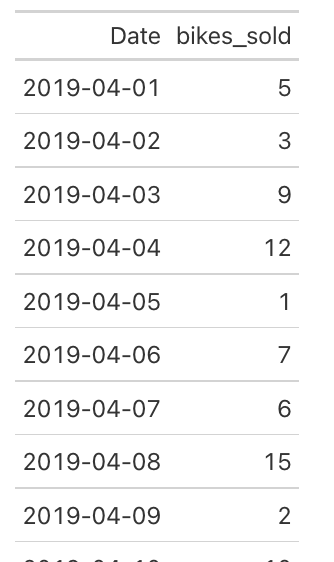
The data includes sales tables of a fictitious bike store for April 2019.

Find the answer to the following questions:

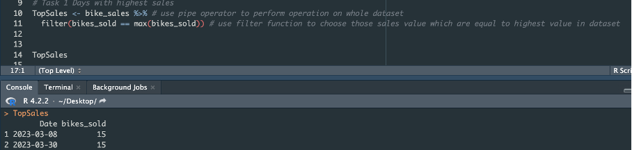
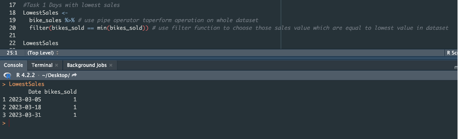
#1.On which day did the store have the highest and lowest sales?

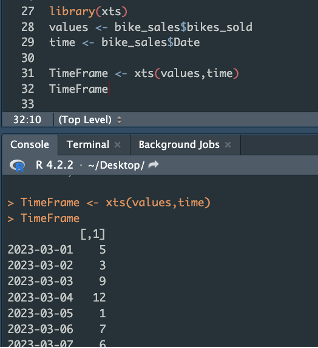
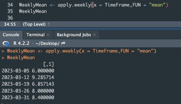
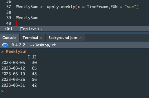
#2.Calculate the average of item sold for every week

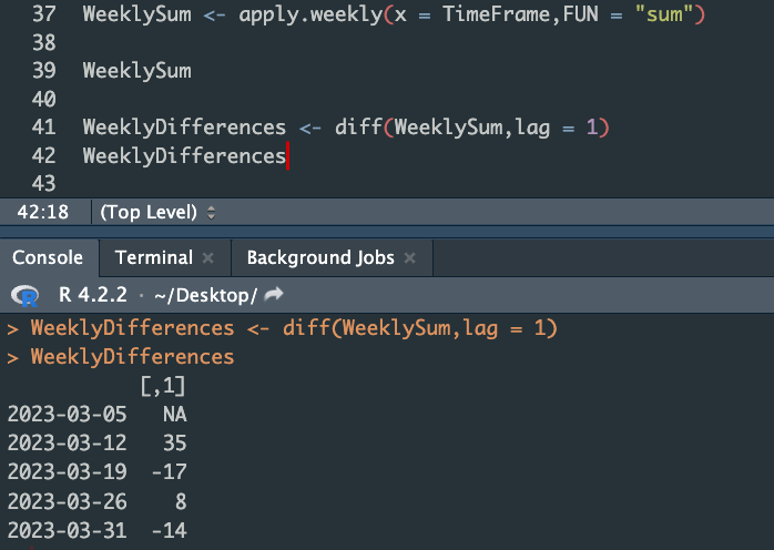
#3.Calculate the difference between sales in consecutive weeks. (For example if first week ended with 100 bikes, and second with 170, answer is 70)

Please be advise that we deal with calendar weeks

#Data

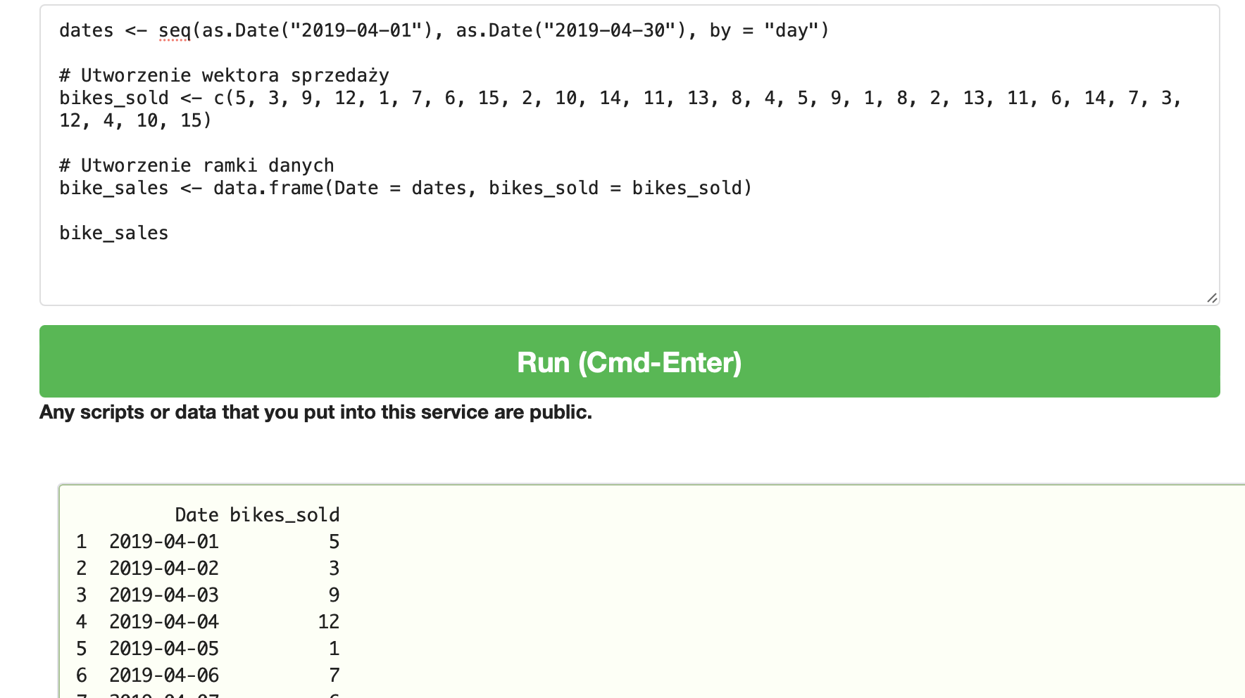
Create vector of dates

dates ← seq(as.Date(“2023-03-01”), as.Date(“2023-03-31”), by = “day”)

Create vector with sold items

bikes_sold ← c(5, 3, 9, 12, 1, 7, 6, 15, 2, 10, 14, 11, 13, 8, 4, 5, 9, 1, 8, 2, 13, 11, 6, 14, 7, 3, 12, 4, 10, 15, 1)

Create data frame

bike_sales ← data.frame(Date = dates, bikes_sold = bikes_sold)

Feel free to use R online: https://rdrr.io/

Submission

Simply post your code and a screenshot of your results.

Please format your R code and blur it or place it in a hidden section.

Solution to this challenge will be posted on May 14

[BrianJ]

@KrzysztofNowak,

Fun challenge - makes you realize how easy the xts package makes working with time series’ and time intelligence calculations.

Here’s my solution:

[KrzysztofNowak]

Thank you for participation.

Below is my solution:

Task 1 Days with highest sales

Solution:

Task 1 Days with lowest sales

Solution:

#2.Calculate the average of item sold for every week

Solution:

For this task we will use xts library. It requires to create xts obiect which take 2 arguments: values and time. Results will be:

There are many useful functions in this package. We will use apply.weekly. It takes 2 arguments: our xts obiect and function we want to apply:

Feel free to experiment with different calendar periods and functions:

#3.Calculate the difference between sales in consecutive weeks. (For example if first week ended with 100 bikes, and second with 170, answer is 70)

You can use same xts obiect, or replace “mean” with “sum”. I will use weekly sum.

Next, I will use diff() function with default lag = 1 parameter. It means that that we compare week to previous one. But we could use different lag value to create interesting analysis.

[KrzysztofNowak]

@BrianJ , i see that we are on the same page;) I just see that for last part You used weekly average, when I used sum. But it is ok, I think that it is good if people will see family of apply. solutions

Regards

[BrianJ]

@KrzysztofNowak ,

Great workout and solution breakdown. The xts package is so powerful and easy to use for time series data. In Power BI, doing previous week calculations (particularly if you’re not using date table offsets) can be a bit of a nightmare, but here it’s as easy as defining your series with a lag.

I just love the simplicity and elegance of R code…