Hi Experts,
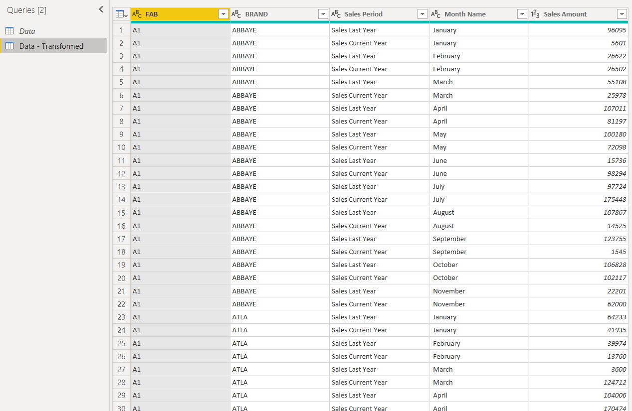
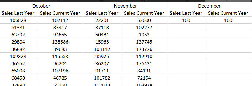
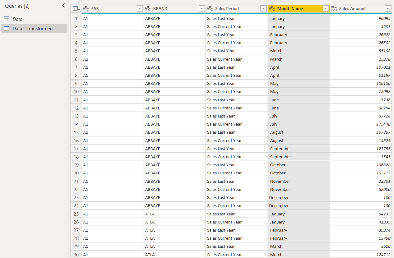
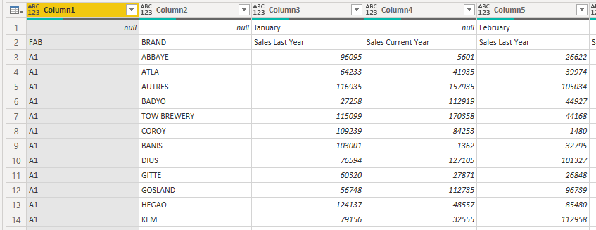
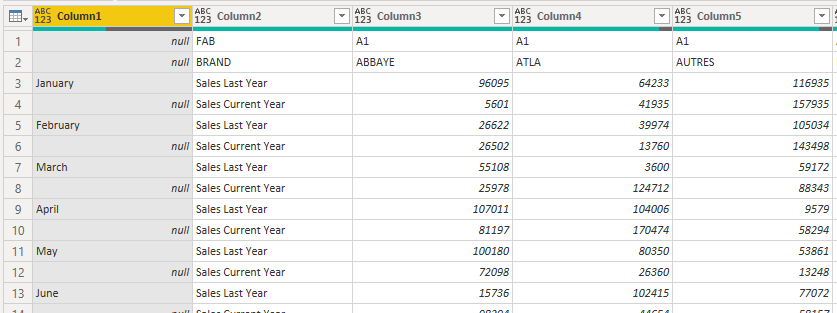
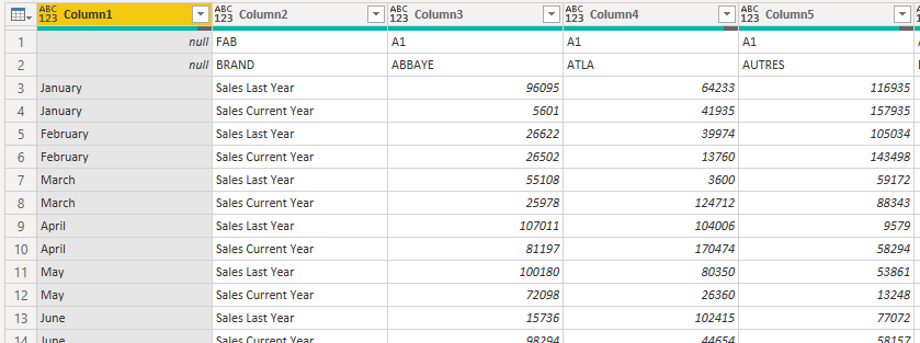
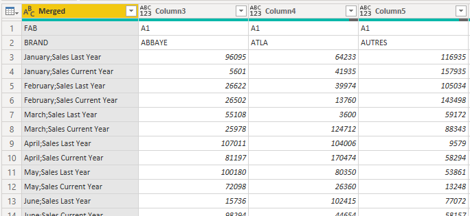
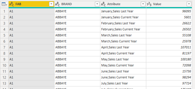
I have the data like below, which is having a merged cell in excel with the Month name, and below it has a current month and previous year sales.
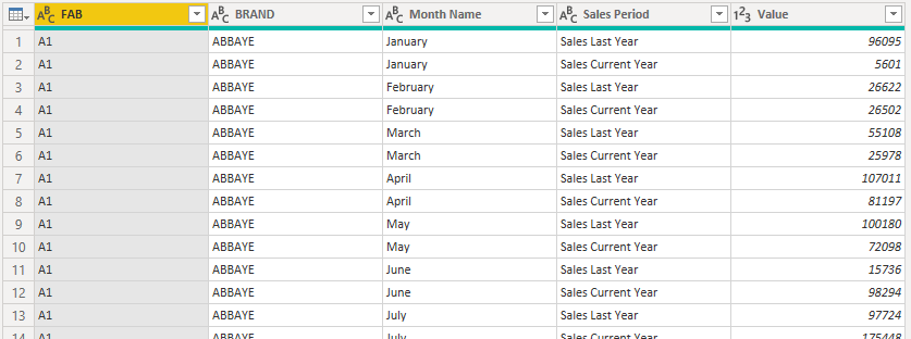
How to do a transformation to use that in the right way in our modeling.
| January | February | March | April | May | |||||||
|---|---|---|---|---|---|---|---|---|---|---|---|
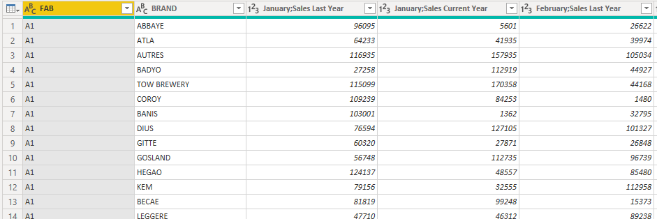
| FAB | BRAND | Sales Last Year | Sales Current Year | Sales Last Year | Sales Current Year | Sales Last Year | Sales Current Year | Sales Last Year | Sales Current Year | Sales Last Year | Sales Current Year |
| A1 | ABBAYE | 96095 | 5601 | 26622 | 26502 | 55108 | 25978 | 107011 | 81197 | 100180 | 72098 |
| A1 | ATLA | 64233 | 41935 | 39974 | 13760 | 3600 | 124712 | 104006 | 170474 | 80350 | 26360 |
| A1 | AUTRES | 116935 | 157935 | 105034 | 143498 | 59172 | 88343 | 9579 | 58294 | 53861 | 13248 |
| A1 | BADYO | 27258 | 112919 | 44927 | 94990 | 60797 | 62528 | 71573 | 98998 | 7560 | 2957 |
| A1 | TOW BREWERY | 115099 | 170358 | 44168 | 127992 | 66873 | 97736 | 39114 | 17056 | 121975 | 58262 |
| A1 | COROY | 109239 | 84253 | 1480 | 69293 | 97402 | 46062 | 107820 | 97966 | 103957 | 17375 |
| A1 | BANIS | 103001 | 1362 | 32795 | 154517 | 47001 | 19970 | 64068 | 60873 | 68479 | 3596 |
| A1 | DIUS | 76594 | 127105 | 101327 | 114456 | 61781 | 162420 | 113287 | 21008 | 62591 | 28487 |
| A1 | GITTE | 60320 | 27871 | 26848 | 5075 | 59793 | 60730 | 114089 | 48054 | 56052 | 167564 |
| A1 | GOSLAND | 56748 | 112735 | 96739 | 138139 | 47958 | 158334 | 99817 | 88347 | 50642 | 25312 |
| A1 | HEGAO | 124137 | 48557 | 85480 | 16783 | 75471 | 139595 | 576 | 164125 | 36792 | 172506 |
| A1 | KEM | 79156 | 32555 | 112958 | 16900 | 76608 | 20195 | 70007 | 67327 | 77239 | 32435 |
| A1 | BECAE | 81819 | 99248 | 15373 | 65913 | 123178 | 85034 | 6606 | 154952 | 108385 | 169816 |
| A1 | LEGGERE | 47710 | 46312 | 89238 | 92939 | 9413 | 4995 | 93437 | 24702 | 125104 | 173479 |
| A1 | STARTOIS | 56833 | 147367 | 111344 | 121096 | 94410 | 46610 | 91348 | 120582 | 79813 | 113729 |
| A1 | TRIPLIET | 100837 | 127617 | 57717 | 170674 | 23792 | 77099 | 104313 | 91428 | 125550 | 153770 |
| B1 | BAVARIN | 63063 | 92799 | 42366 | 132047 | 20686 | 116533 | 116164 | 72335 | 2554 | 128702 |
| B1 | AUTREB | 120837 | 27711 | 15697 | 1110 | 48437 | 36329 | 96019 | 34832 | 87138 | 60841 |
| B1 | HORNET | 74000 | 130077 | 76253 | 99041 | 40793 | 131722 | 94840 | 149843 | 68990 | 155051 |
| B1 | OTHER BRANDS | 19325 | 77554 | 107378 | 154102 | 19425 | 97013 | 42593 | 137633 | 50687 | 120409 |
| B1 | PALM | 45852 | 98902 | 53434 | 56056 | 117072 | 131840 | 40096 | 35876 | 63553 | 64919 |
| B1 | RODENCH | 45883 | 163506 | 108343 | 90751 | 83005 | 154700 | 24750 | 71039 | 45759 | 1918 |
| B1 | STEENBRU | 110901 | 138101 | 56587 | 96039 | 87910 | 80629 | 85415 | 31229 | 108982 | 141907 |
| B1 | URTHEL | 78341 | 138376 | 110179 | 20939 | 46580 | 143507 | 107703 | 117738 | 47839 | 107389 |
| G1 | 1765 | 36962 | 159422 | 80068 | 78516 | 95092 | 103871 | 100482 | 47483 | 108491 | 114691 |
| G1 | TRESSBERG | 54333 | 18138 | 99143 | 33843 | 110800 | 146952 | 5738 | 2094 | 12560 | 43305 |
| G1 | BROOK | 111545 | 24979 | 38215 | 111243 | 106348 | 94775 | 53908 | 128713 | 10312 | 6249 |
Attaching the excel file for your reference.Data Transfer.xlsx (19.9 KB)
Any quick will be greatly appreciated.
Thanks


 - I guess now you converted me from a normal Indian guy to a specific South Indian one.