Lowest Net Revenue Locations

[jmwdba]

So using RANKX I am showing the lowest net revenue locations and in another table the highest net revenue locations. The problem is instead of showing the Lowest 10, it only shows the lowest 8 and I cannot figure out why it stops at 8 instead of showing 10.

My Lowest Net Revenue Formula is:

Lowest Net Revenue = 
    VAR
        RankingDimension = VALUES( 'WW Fiscal Locations'[Fiscal Location Name])
    VAR
        RankingSelect = [Lowest Ranking Select]
    RETURN
        CALCULATE( [Net Revenue],
            FILTER(RankingDimension,
                RANKX(ALL('WW Fiscal Locations'[Fiscal Location Name]), [Net Revenue], , ASC) <= RankingSelect))

Net Revenue is calculated by:
Net Revenue = [Total Revenue from Tuition] - [Overall Expenses]

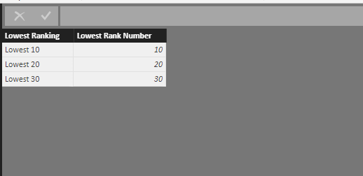
Lowest Ranking Select is:

Lowest Ranking Select = IF( HASONEVALUE( 'Lowest Ranking'[Lowest Ranking]), VALUES( 'Lowest Ranking'[Lowest Rank Number] ), 1000000)
//select the rank number based on slicer selection

My Lowest Ranking Table is as follows:

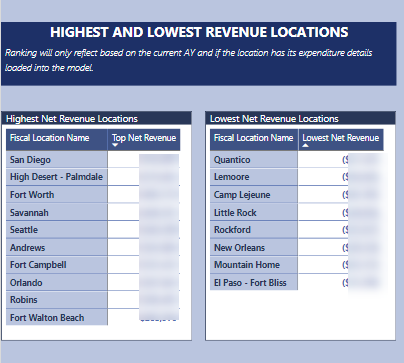
Of course I had to blur out the actual net revenues but below is the visual. The Highest Net Revenue Locations visual shows a perfect 10 locations as expected but the lowest only shows 8 instead of 10. Is there something that only makes it show lowest if the lowest is negative?

[jmwdba]

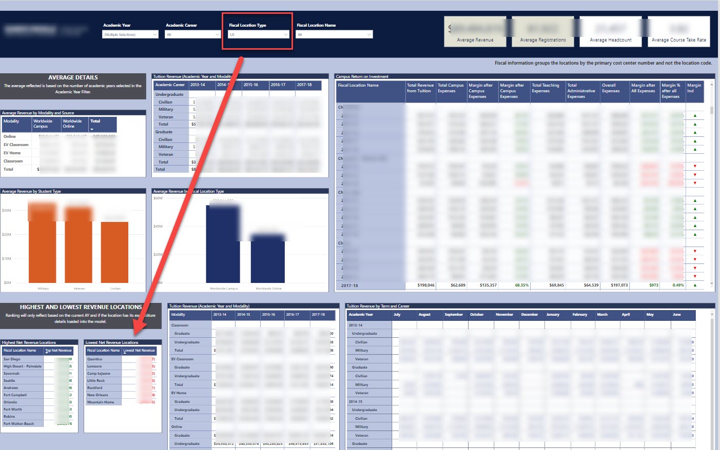
One additional note. So I notice when I have it set to show both US and International Locations it shows a perfect bottom 10 locations. When I have a filter set to show only US locations thats when it only shows 8. Is it possible to make it show the bottom 10 locations specific to the US Location filter being applied?

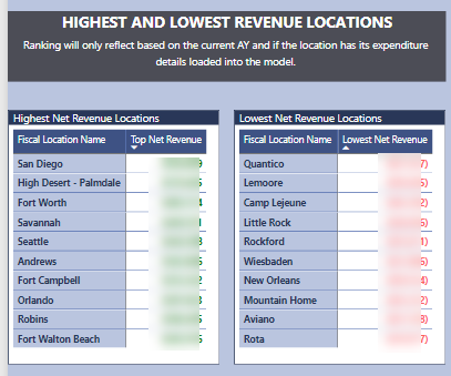
This is what shows when I have the top filter set to show both US and International Campus Locations:

[sam.mckay]

Yes that’s immediately what I would have thought, that an additional filter was in place.

To adjust this so that it works with your filtering you need to change the ALL() part of the RANKX formula.

You likely don’t want the specific column but the entire table.

So instead of this

ALL('WW Fiscal Locations'[Fiscal Location Name])

You likely need this

ALL('WW Fiscal Locations')

Can you try this and see how it goes.

Also it a good opportunity to really think what’s happening with the calculation and why the ALL is required in the first place. It’s an interesting thing to think about.

Also another help is in the table to actually see the rank number. Then you can quickly audit why it is or isn’t showing.

Sam

[jmwdba]

This makes sense. I tried it and it didn’t change the outcome. It’s almost like it only includes it in the lowest if the amount is negative as it captures all of the negative net revenues but when looking specifically at the US locations exclusively then it should include 3 that are positive net revenues but they are small like one location only have $973 dollars in positive revenue.

But there is no logic in the formula that tells it to only look for Net Revenue thats negative.

[sam.mckay]

Where you able to actually just place the ranking number next to that result and audit it that way.

Being able to actually see the numbers will tell you quite a lot about what the calculation is doing.

What I would do it break this out into another testing page and just focus on this one formula. Then break out each part of it and analyze what it is calculating when different filters are in place.

I always do this - I’ve found it’s the best way to learn the behaviour of more complex formula.

Chrs