Hello @Vladas,
Thank You for posting your query onto the Forum.
Well that firstly, I would like to state the following reasons “Why” it’s not working for you.
-
The “Rules” table that you’ve created is comparing the “Column Names” with the individual “Row Name” of the “Item List” table in the case of “Suppliers” and then it’s comparing “TypeID’s” at a row level. The dynamics of the itself is bit unorthodox.
-
Due to this, firstly, you cannot compare “Column Headers” with the individual row level items in the formula.
-
The naming conventions for the “SupplierA” and “SupplierB” is only same between the two tables and then “SupplierC”, “SupplierD”, “SupplierF” and “SupplierG” is being combined under the one roof i.e. “Other Suppliers”. Due to difference in naming conventions how will the formula be able to distinguish what’s what?
-
Other thing is second table i.e. “Rules” table which you’ve created is just being used to extract the percentages and then accordingly calculate the “Sales Price” but in order to do that firstly, the items from that table as well need to be used/put/dragged somewhere into the table visualization so that we can use the “SELECTEDVALUE()” function. Right now, due to this circumstances Power BI is not able to identify which percentage to select for which category.
-
This type of tables are mostly applicable in the case of “Scenario Analysis” where you want to analyze and change the “Sales Price” depending upon the range/criteria selected or if you’re using the tables as a “Filter/Slicer” option.
Therefore, after considering all these points, what you can simply do is put this percentage criteria’s directly into the formula in order to calculate the “Sales Price”. Below is the formula provided for the reference -
-
Calculate the “Cost Price” -
Cost Price - Harsh = SUM( ItemList[Cost price] )
-
Calculate the “Sales Price” for each individual line items -
 New Sales Price - Harsh 1 =
 SWITCH( TRUE() ,
     SELECTEDVALUE( ItemList[TypeId] ) = "Type1" && SELECTEDVALUE( ItemList[Supplier] ) = "SupplierA" ,
         [Cost Price - Harsh] + ( [Cost Price - Harsh] * 0.2 ) ,
     SELECTEDVALUE( ItemList[TypeId] ) = "Type2" && SELECTEDVALUE( ItemList[Supplier] ) = "SupplierA" ,
         [Cost Price - Harsh] + ( [Cost Price - Harsh] * 0.3 ) ,
     SELECTEDVALUE( ItemList[TypeId] ) = "Type3" && SELECTEDVALUE( ItemList[Supplier] ) = "SupplierA" ,
         [Cost Price - Harsh] + ( [Cost Price - Harsh] * 0.4 ) ,
     SELECTEDVALUE( ItemList[TypeId] ) = "Type4" && SELECTEDVALUE( ItemList[Supplier] ) = "SupplierA" ,
         [Cost Price - Harsh] + ( [Cost Price - Harsh] * 0.5 ) ,
     SELECTEDVALUE( ItemList[TypeId] ) = "Type5" && SELECTEDVALUE( ItemList[Supplier] ) = "SupplierA" ,
         [Cost Price - Harsh] + ( [Cost Price - Harsh] * 0.6 ) ,

     SELECTEDVALUE( ItemList[TypeId] ) = "Type1" && SELECTEDVALUE( ItemList[Supplier] ) = "SupplierB" ,
         [Cost Price - Harsh] + ( [Cost Price - Harsh] * 0.6 ) ,
     SELECTEDVALUE( ItemList[TypeId] ) = "Type2" && SELECTEDVALUE( ItemList[Supplier] ) = "SupplierB" ,
         [Cost Price - Harsh] + ( [Cost Price - Harsh] * 0.65 ) ,
     SELECTEDVALUE( ItemList[TypeId] ) = "Type3" && SELECTEDVALUE( ItemList[Supplier] ) = "SupplierB" ,
         [Cost Price - Harsh] + ( [Cost Price - Harsh] * 0.7 ) ,
     SELECTEDVALUE( ItemList[TypeId] ) = "Type4" && SELECTEDVALUE( ItemList[Supplier] ) = "SupplierB" ,
         [Cost Price - Harsh] + ( [Cost Price - Harsh] * 0.75 ) ,
     SELECTEDVALUE( ItemList[TypeId] ) = "Type5" && SELECTEDVALUE( ItemList[Supplier] ) = "SupplierB" ,
         [Cost Price - Harsh] + ( [Cost Price - Harsh] * 0.8 ) ,

     SELECTEDVALUE( ItemList[TypeId] ) = "Type1" ,
         [Cost Price - Harsh] + ( [Cost Price - Harsh] * 0.35 ) ,
     SELECTEDVALUE( ItemList[TypeId] ) = "Type2" ,
         [Cost Price - Harsh] + ( [Cost Price - Harsh] * 0.45 ) ,
     SELECTEDVALUE( ItemList[TypeId] ) = "Type3" ,
         [Cost Price - Harsh] + ( [Cost Price - Harsh] * 0.55 ) ,
     SELECTEDVALUE( ItemList[TypeId] ) = "Type4" ,
         [Cost Price - Harsh] + ( [Cost Price - Harsh] * 0.65 ) ,
     SELECTEDVALUE( ItemList[TypeId] ) = "Type5" ,
         [Cost Price - Harsh] + ( [Cost Price - Harsh] * 0.75 ) )
-
Lastly, in order to calculate the “Grand Totals” as well. Here’s the formula for the reference -
 New Sales Price - Harsh 2 =
 SUMX(
     SUMMARIZE(
         ItemList ,
         ItemList[ItemName] ,
         ItemList[TypeId] ,
         ItemList[Supplier] ,
         "Grand Totals" ,
         [New Sales Price - Harsh 1] ) ,
 [Grand Totals] )
A quick note here: You can also achieve this within the single formula (Using: VariablesTechnique), but due to length of the formula I’ve created another measure (Using: Measure Branching Technique) just for the simplification purpose.
General Tip: Whenever you want to create a Table, rather than using the “Enter Data” option from the “Home Tab” you can create a same table using the “New Table” option available under the “Modelling” tab. The main advantage of doing is using the “New Table” you can create a table using the formulas wherein in future if you want to change any figure you’ll be easily able to do that but this option is not available under the “Enter Data” option. Once you create a data/table using this option it gets fixed into the model and changes cannot be made.
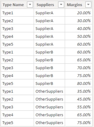
So here’s the formula’s that I’ve written to create that “Rules” table wherein you can change the naming conventions and figures, if required in future.
This table can still prove to be a helpful to identify what percentages were put in the formula while calculating the “Sales Price” (for reference).
Rules - Harsh =
UNION(
    ROW( "Type Name" , "Type1" , "Suppliers" , "SupplierA" , "Margins" , 0.2 ) ,
    ROW( "Type Name" , "Type2" , "Suppliers" , "SupplierA" , "Margins" , 0.3 ) ,
    ROW( "Type Name" , "Type3" , "Suppliers" , "SupplierA" , "Margins" , 0.4 ) ,
    ROW( "Type Name" , "Type4" , "Suppliers" , "SupplierA" , "Margins" , 0.5 ) ,
    ROW( "Type Name" , "Type5" , "Suppliers" , "SupplierA" , "Margins" , 0.6 ) ,

    ROW( "Type Name" , "Type1" , "Suppliers" , "SupplierB" , "Margins" , 0.6 ) ,
    ROW( "Type Name" , "Type2" , "Suppliers" , "SupplierB" , "Margins" , 0.65 ) ,
    ROW( "Type Name" , "Type3" , "Suppliers" , "SupplierB" , "Margins" , 0.7 ) ,
    ROW( "Type Name" , "Type4" , "Suppliers" , "SupplierB" , "Margins" , 0.75 ) ,
    ROW( "Type Name" , "Type5" , "Suppliers" , "SupplierB" , "Margins" , 0.8 ) ,

    ROW( "Type Name" , "Type1" , "Suppliers" , "OtherSuppliers" , "Margins" , 0.35 ) ,
    ROW( "Type Name" , "Type2" , "Suppliers" , "OtherSuppliers" , "Margins" , 0.45 ) ,
    ROW( "Type Name" , "Type3" , "Suppliers" , "OtherSuppliers" , "Margins" , 0.55 ) ,
    ROW( "Type Name" , "Type4" , "Suppliers" , "OtherSuppliers" , "Margins" , 0.65 ) ,
    ROW( "Type Name" , "Type5" , "Suppliers" , "OtherSuppliers" , "Margins" , 0.75 ) )
Note: You can change the dynamics of the table. i.e. you can also represent the table the way you’ve created using the “Enter Data” option. I’ve just shown it for example purpose.
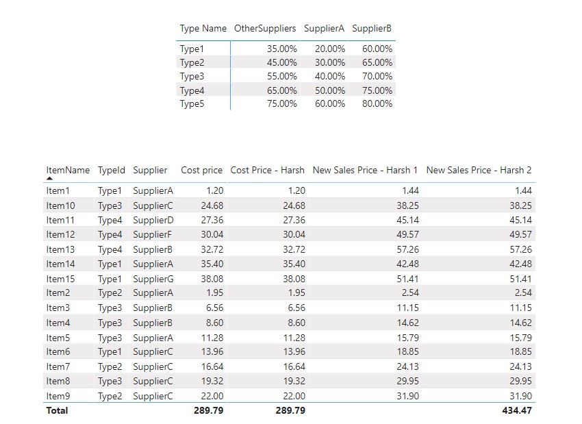
So lastly, here’re the end results. Below are the screenshots provided for the reference -
After a lengthiest explanation, you might want to consider looking at a file more in-depth. So I’m also attaching the working of the PBIX file for the reference.
Hoping you find this useful and meets your requirements that you’ve been looking for. 
Thanks and Warm Regards,
Harsh
Supplier.pbix (38.3 KB)