Welcome to Excel Workout #7!
Difficulty Level:

This week’s challenge is designed to test your knowledge on Conditional Formatting.
Conditional Formatting
Conditional Formatting in Excel is a feature that allows users to format cells based on specific conditions or criteria. It is a powerful tool that helps to highlight important data or identify patterns in large data sets.
With conditional formatting, users can apply different formatting styles to cells based on the value of the cell, the content of the cell, or the comparison of the cell value to other cells. For example, a user can apply a specific color to cells that contain values greater than a certain number or apply a different color to cells that contain specific text.
Goals
Please follow the directions given below, which include downloading the Excel worksheet required to perform the challenge tasks. Once you have completed the download, proceed to take the challenge and test your skills.
Task
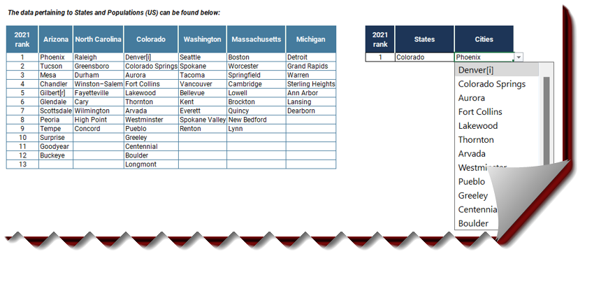
State names located in the Y4:AD4 range can be selected from the Drop-Down menu in AG5 Cell.
Let’s choose Arizona from cell AG5.
Cities belonging to the State of Arizona in cell AH5 will be listed in the drop-down list.
Let’s pick the city of Phoenix.
Again, let’s select the State of Colorado from cell AG5.
The city of Phoenix is still visible in cell AH5 whereas, the city of Phoenix belongs to the Arizona State.
When we click the drop-down button in cell AH5, we only know the Colorado state cities by sight.
The question is:
When we change the States in cell AG5, how can we ensure that the value in cell AH5 is blank until the new city is selected?
Submission
Reply to this post with your formula code and solution file. Please be sure to blur or hide your formula code.
Period
This workout will be released on Monday April 17, 2023 , and the author’s solution will be posted on Sunday April 23, 2023 .
Challenge #7.xlsx (8.3 MB)
Good luck,
Ilgar Zarbaliyev
1 Like
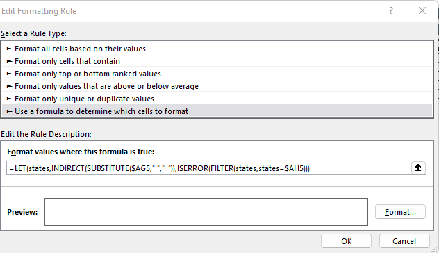
The cities column were selected to apply the conditional formatting.
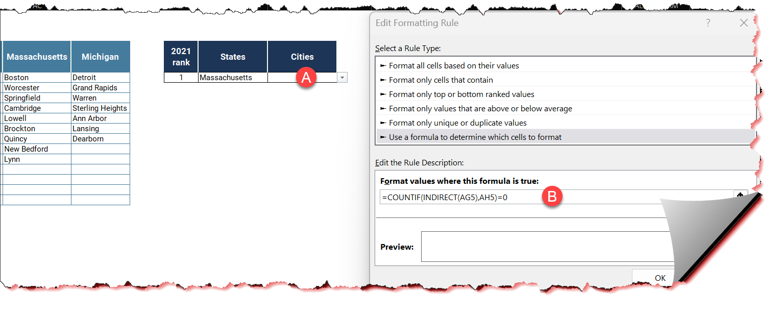
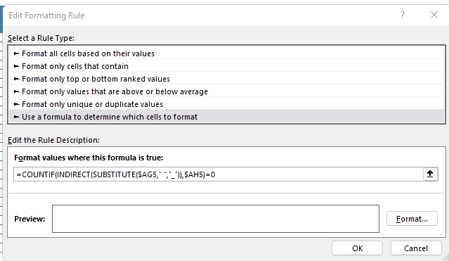
Here I select the "use a formula to determine which cells to format.
The formula used here is
=LET(states,INDIRECT(SUBSTITUTE($AG5," ","_")),ISERROR(FILTER(states,states=$AH5)))
The formula used here is to filter the cities in the cities column by state and check if the cities belongs to the state. If it does not it will return an error. Hence, the need for the ISERROR() function . So once the condition is “TRUE”.
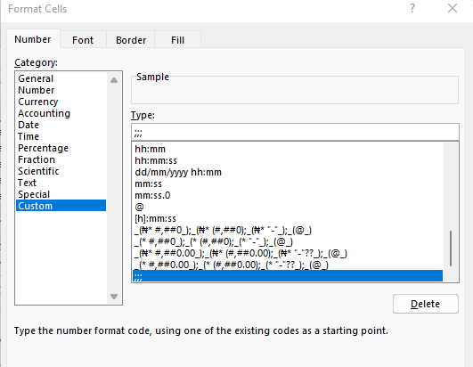
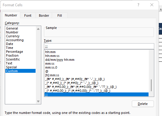
Then , I proceeded to do a custom number formatting. I replaced the “General” which is the default to ;;; which means the cells should display blank
Quadri Atharu - Challenge #7 Solution.xlsx (8.3 MB)
1 Like
Formula
=COUNTIF(INDIRECT(SUBSTITUTE($AG5," ","_")),$AH5)=0
`
Quadri Atharu - Challenge #7 2nd Solution.xlsx (8.3 MB)
1 Like
I will use this approach for solving it.
- Create a conditional formatting formula
=COUNTIFS(XLOOKUP(AG5, Y4:AD4, Y5:AD17), AH5)
- Use the following cell formatting in the Conditional Formatting options.
;;;;
We can also use VBA to reset the cell, but that will come with the troubles of .xlsm file.
Challenge #7.xlsx (8.3 MB)
2 Likes
An awesome use of XLOOKUP Aditya. You’ve tempted me to try one more formula despite resisting the urge.
1 Like
Alternative Formula
Conditional Formatting Formula
=SUM(N(FILTER(Y5:AD17,Y4:AD4=AG5)=AH5))=0
Custom number formatting - ;;;
3rd Solution Challenge #7.xlsx (8.3 MB)
1 Like
Thank you for your versions…
However, I will solve this challenge using simple CountIf function and Conditional Formatting…Very simple…
1 Like
A little hint please? I don’t want to look at solutions. Is it the IN operator? Something like if the cities in the states?
1 Like
Sure…We can use Countif Function for the solution of this workout.
The formula then will be used in Conditional Formatting.
Number Formatting like “;;;” will be also used.
I am not sure in what context it can be considered as a hint. However, I think it can help.
Thank you for participating in the Excel Challenge related to Name Manager, Data Validation and Indirect Function! I hope you found this challenge to be a fun and engaging way to improve your Excel skills and learn more about how to perform conditional formatting in Excel.
Here is my solution to Workout #7:
=COUNTIF(INDIRECT(AG5),AH5)=0
We hide the value of the first element of the list with
conditional formatting and assigned a format of either red
color or assigned a custom one - “;;;”.
Challenge #7 with Solution.xlsx (8.4 MB)
Once again, thank you for participating in this Excel Challenge, and I look forward to seeing you in future challenges and learning opportunities!
To be honest, it was quite tricky and didn’t get it well initially so I had to look up my peers’ responses.
Thanks, @QuadriAtharuOlayinka and @HermioneGranger1176 for the guidance.
I understand the logic well now.
Sharing the workbook:
C7_ConditionalFormatting_Homesh.xlsx (47.9 KB)
2 Likes
You’re welcome @homesh_agarwal
1 Like
@IlgarZarbaliyev - While these workouts were closed a long time ago, practicing them certainly enhanced my knowledge.
Here’s my workout file - Challenge #7.xlsx (8.3 MB)
1 Like