I found a work-around, but it’s not working on the total row (and I don’t have time to handle that part, so I’m going to leave that to you)
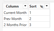
First - you DO need to be dealing with a Matrix, and your visual is a table. I solved this by creating a Colum Map table for your three columns.
You can match the original measure names if you want, this is just what I chose.
Next - you need a measure to map the three sales measures over to this new table:
Sales Amount =
VAR _SelectedColumn = SELECTEDVALUE( 'Matrix Column Map'[Column] )
RETURN
    SWITCH( TRUE(),
        _SelectedColumn = "Current Month", [Sales],
        _SelectedColumn = "Prev Month", [Prev Month Sales],
        _SelectedColumn = "2 Months Prior", [Prev 2MONTHS SALE])
then, you need a measure to handle the formatting (I actually created three - but you’ll need only one or two depending on how you choose to handle the conditional format rule)
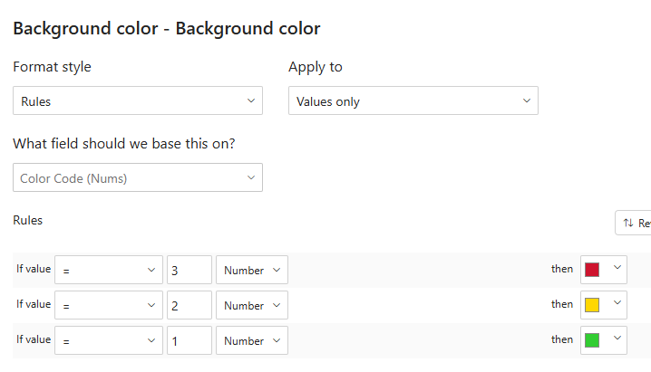
if you want to handle the formatting like this:
Create the Color Code (Nums) measure
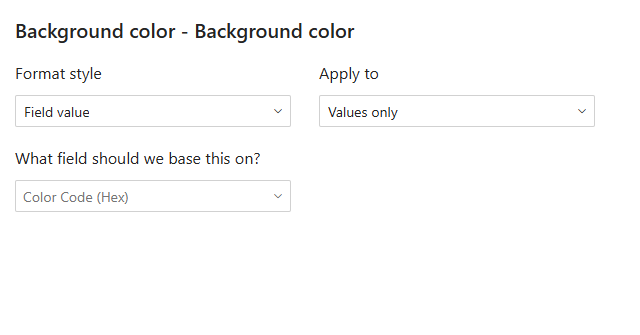
if you want to handle the formatting like this:
Create two measuers, one for the background (Color Code Hex), and one for the font (Font Color Hex). Personally this second method is my preference, because I can use it in multiple tables if needed and only update the measure if I want the color to change.
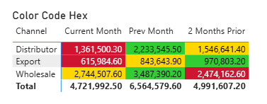
Color Code (Hex) =
VAR _MaxValue =
    MAXX(
        { [Sales], [Prev 2MONTHS SALE], [Prev Month Sales] },
        [Value] )
VAR _MinValue =
    MINX(
        { [Sales], [Prev 2MONTHS SALE], [Prev Month Sales] },
        [Value] )
RETURN
    SWITCH( TRUE(),
        [Sales Amount] = _MaxValue, "#32CD32",
        [Sales Amount] = _MinValue, "#CE142E",
        "#FFD700")
the formulas are similar, so only showing one here.
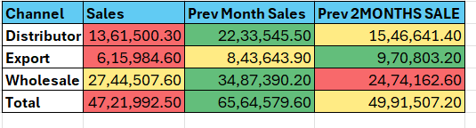
and your outcome is:
both versions are demonstrated in the attached file.
eDNA Solution - Matrix Conditional Row Format.pbix (337.0 KB)