Aggregating customer purchases by Month

[pete.langlois]

I have a trickey request from a client that I would love some help with. Here’s what’s going on:

Im using a standard transaction table, which contains the following columns, among others:

Date
Year and Month
Sale Amount
Customer Name

I would like to create another column on this transaction that summarizes the sales by month and customer name. For reasons I explain below, I cannot use the summarizecolumn function in order to create a new table that accomplishes this same task. I need those values to exist on the original transaction table.

I’ve attached an excel doc which shows an example of what I’m trying to accomplish. You’ll see 4 columns highlighted green which I already have in the table. The yellow highlighted columns (which summarize the sales amount by month and customer name and then place those new aggregated values into buckets using switch true ) is what I’m trying to accomplish with a calculated column so it sits on the same transaction table.

Why not create a new table with summarizecolumns?

My actual transaction table contains a variety of other columns (item type, customer type, color, etc.), which I need to use to filter the report. My client said they consider every purchase that occurs for each customer during a single month to be a single purchase, even if it shows up as 6 individual records in the transaction table. For example, if customer A purchase 6 different items throughout the month of January 2020 for $5 per item, those 6 purchases are considered a single purchase of $30. Even if the items are of different item type and color, they are to be considered a single purchase.

The client then wants me to place these new aggregated purchase amounts (aggregated by customer and month) into buckets of 1-5, 6-10, 11-25, etc. The client then wants to be able to gather some insights from these buckets for example, what % of sales come from purchases that fit into the $501-1000 bucket.

I tried using the summarizecolumn function, but when but I wasn’t able to filter from the new virtual table back onto the original transaction table due to circular redundancy.

So, if anyone knows how to accomplish this, please help!!!

dummy data.xlsx (12.1 KB)

[BrianJ]

@pete.langlois,

Power Query eats these kind of grouping problems for breakfast. Check out how easily it handles this one:

Here’s the step that does most of the heavy lifting:

let
    Source = RawData,
    #"Changed Type" = Table.TransformColumnTypes(Source,{{" Sales Amount ", Currency.Type}}),
    #"Grouped Rows" = Table.Group(#"Changed Type", {"Customer", "Year and month"}, {{"AllData", each _, type table [index=nullable number, Customer=nullable text, date=nullable date, Year and month=nullable date, #" Sales Amount "=nullable number]}, {"TotSales", each List.Sum([#" Sales Amount "]), type nullable number}}),
    #"Removed Columns" = Table.RemoveColumns(#"Grouped Rows",{"Customer", "Year and month"}),
    #"Expanded AllData" = Table.ExpandTableColumn(#"Removed Columns", "AllData", {"index", "Customer", "date", "Year and month", " Sales Amount "}, {"index", "Customer", "date", "Year and month", " Sales Amount "}),
    #"Added Conditional Column" = Table.AddColumn(#"Expanded AllData", "Bucket", each if [TotSales] >= 50 then "50+" else if [TotSales] >= 26 then "26  - 50" else if [TotSales] >= 11 then "11 - 25" else if [TotSales] >= 6 then "6 - 10" else "1 - 5", type text)
in
    #"Added Conditional Column"

I hope this is helpful. Full solution file attached below.

– Brian
eDNA Forum - Aggregate Sales Buckets Solution.pbix (29.6 KB)

[pete.langlois]

Hey Brian, thanks for your solution. I was able to generate a similar result using the summarizecolumn function. My goal isn’t to create a new table, however, rather to add some aggregations onto the existing fact table.

Put another way:

Imagine my base fact table contains the following 5 columns only (highlighted green in my dummy data):

index
customer
date
year and month
sales amount

How do I use dax to create the 2 new columns with the same data from my dummy data excel doc (yellow highlighted in dummy data)?

Totsales by customer and month
Buckets

Imagine that the columns from my dummy data “total sales by customer and month” and “buckets” don’t exist, so I need to somehow create them so the data matches what I put in the dummy data example. In my example, the green columns are what I’m starting with, and the yellow columns are what I am trying to create FROM the green columns.

Hopefully this makes sense…

@Harsh Any ideas?

[BrianJ]

@pete.langlois,

Check out the revised file. I think it does exactly what you’re requesting - takes only the initial five columns from the Excel file (I’ve deleted the other columns in the attached Excel file just for clarity), creates the sales aggregations by month and customer and creates the five buckets. Does so leaving only one table with the original five columns and the two additional.

I hope this hits the mark. PBIX and Excel files attached.

• Brian
  eDNA Forum - Aggregate Sales Buckets Solution2.pbix (44.9 KB) dummy data.xlsx (11.6 KB)

[EnterpriseDNA]

Hi @pete.langlois, did the response provided by @BrianJ help you solve your query? If not, how far did you get and what kind of help you need further? If yes, kindly mark as solution the answer that solved your query. Thanks!

[EnterpriseDNA]

Hi @pete.langlois, we’ve noticed that no response has been received from you since the 25th of February. We just want to check if you still need further help with this post? In case there won’t be any activity on it in the next few days, we’ll be tagging this post as Solved.

[EnterpriseDNA]

Hi @pete.langlois, a response on this post has been tagged as “Solution”. If you have a follow question or concern related to this topic, please remove the Solution tag first by clicking the three dots beside Reply and then untick the check box.

We’ve recently launched the Enterprise DNA Forum User Experience Survey, please feel free to answer it and give your insights on how we can further improve the Support forum. Thanks!

[pete.langlois]

Thanks, Brian! I’ve been out of town so sorry for the delay in responding.

Can you walk me through the “grouped rows” step, then the expanded data steps? These 2 steps seem to be where the magic happens, but I’m not sure how you got there. I tried using “Group by” but it created a new table without the option to expand the data. Perhaps I’m inputting the wrong column names in the fields…Feeling a bit lost.

Thanks again!

[BrianJ]

@pete.langlois,

I can tell from your question that you’re actually quite close here, but are missing one secret ingredient. Let me show you.

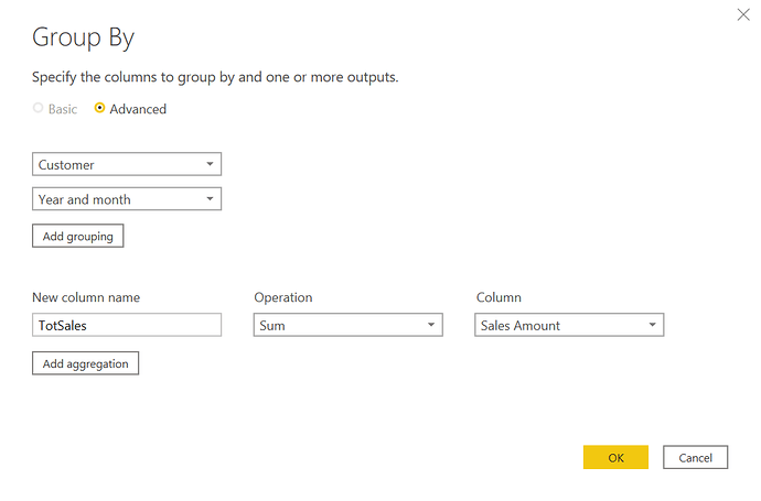
Typically the way Groupby works is that it groups on a series of fields you specify, and then creates an additional column or columns with aggregate calculations based on these groupings. So in your dataset, if we group on customer and month and then aggregate on sales, the grouping function will look like this:

and will produce this result:

This is what you asked Power Query to do, but not what you want – instead you want to retain ALL the rows of your original table and put the aggregate results for each grouping onto each row of the table.

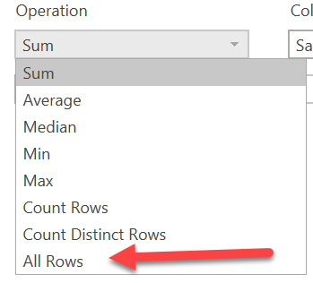
You may have noticed when you selected the SUM aggregate function, that there was one weird, nonintuitive selection at the bottom called “All Rows”. This is the special sauce that makes GroupBy so powerful.

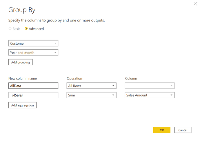
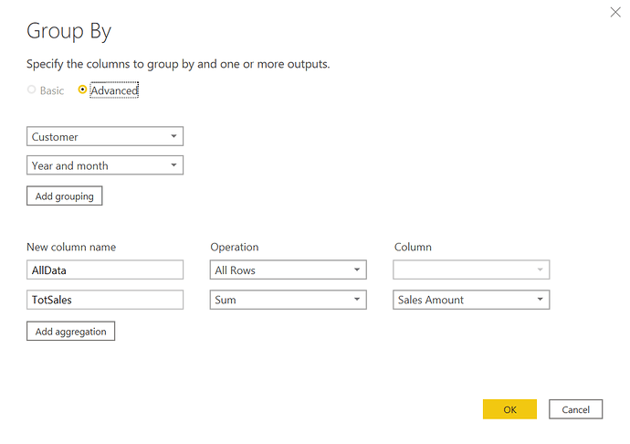
What this does is tells Power Query to retain ALL the rows of your original table, perform the aggregation and place that result on EACH row within the distinct grouping you defined – exactly the result you are looking for. Here’s what the revised grouping configuration looks like:

And here’s what the result looks like after you expand, making sure to uncheck the columns you originally grouped on so that they don’t get duplicated:

Once you know this trick, I think you’ll find that every time you see the need to group and aggregate this will become your go-to option since IMO this is much easier than writing the comparable DAX.

I hope this clarifies things and gives you an excellent new tool in your toolbox. Give a shout if you still have questions.

– Brian

[pete.langlois]

Amazing, thank you!