Excel Workout 6 - Offset Function

IlgarZarbaliyev · April 13, 2023, 4:28am

Welcome to Excel Workout #6!
Difficulty Level:

This week’s challenge is designed to test your knowledge on Offset function.

Offset Function
The OFFSET function is a built-in function in Microsoft Excel that allows you to reference a cell or a range of cells that are located a specified number of rows and columns away from a starting cell or range. The OFFSET function is commonly used in dynamic formulas and charts where the range of data changes frequently.

Goals
Please follow the directions given below, which include downloading the Excel worksheet required to perform the challenge tasks. Once you have completed the download, proceed to take the challenge and test your skills.

Task
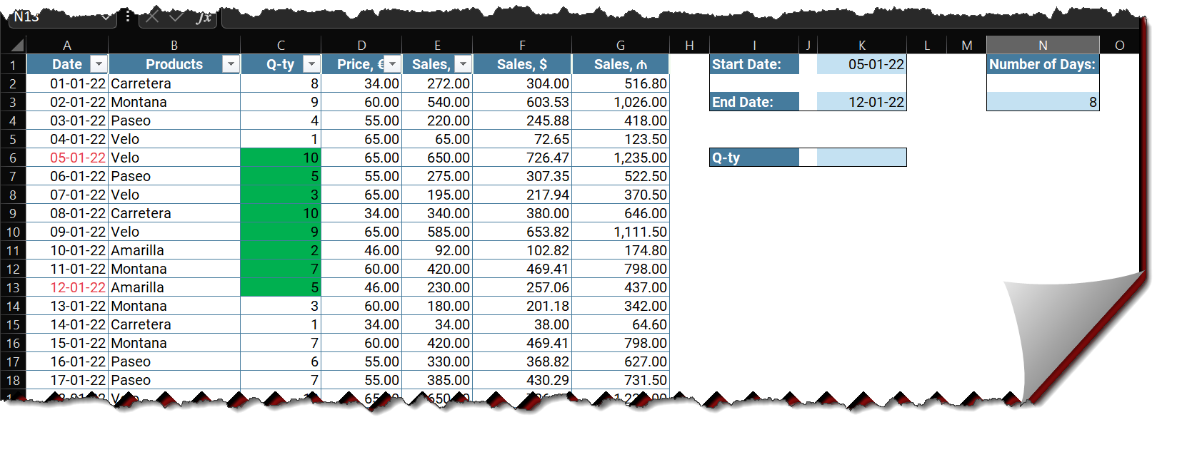
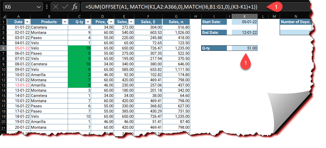
In cell K6, create a formula utilizing the OFFSET function to ascertain the sum value for the chosen field value (I6 cell), taking into account the start and end dates (K1:K3 cells).

Submission
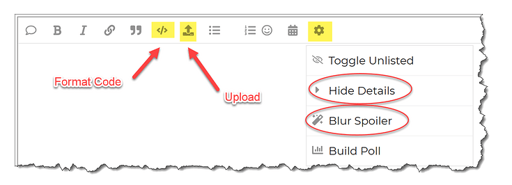
Reply to this post with your formula code and solution file. Please be sure to blur or hide your formula code.

Period
This workout will be released on Thursday April 13, 2023, and the author’s solution will be posted on Wednesday April 19, 2023.

Challenge #6.xlsx (8.3 MB)

Good luck,

Ilgar Zarbaliyev

QuadriAtharuOlayinka · April 13, 2023, 7:48am

Formula Solution

Having gone through the task requirement all over again, I understood there’s no need to consider product as a field. Then I’ll stick with my initial formula. Which is to sum values rather than looking for ways to count products.


=SUM(OFFSET(INDEX(A1:G1,MATCH(I6,A1:G1,0)),MATCH(K1,A2:A366,0),,K3-K1+1))

Formula Breakdown

MATCH(I6,A1:G1,0) - This returns the relative position of the chosen field in I6 within the A1:G1.

OFFSET is used to return ranges based on the starting date and end date.

There are also several ways to go about this as well just like in the other workouts. Ideally I would have gone with an XLOOKUP, or other dynamic array formulas as it also return ranges. OFFSET is known to be volatile but it’s still a powerful function.

One alternative way to solve this without Offset is:


> =SUM(FILTER(CHOOSECOLS(A2:G366,XMATCH(I6,A1:G1)),(A2:A366>=K1)*(A2:A366<=K3)))

Quadri Atharu Challenge #6 - Offset Solution.xlsx (8.3 MB)

HermioneGranger1176 · April 13, 2023, 9:58am

Here are a few ways to do it in Excel. I have not used the OFFSET function in any of them.

=IFNA(
    SUMIFS(XLOOKUP(I6, C1:G1, C2:G366), A2:A366, ">=" & K1, A2:A366, "<=" & K3),
    K3 - K1 + 1
)

=IFNA(
    SUM(
        XLOOKUP(K1, A2:A366, XLOOKUP(I6, C1:G1, C2:G366)):
            XLOOKUP(K3, A2:A366, XLOOKUP(I6, C1:G1, C2:G366))
    ),
    K3 - K1 + 1
)

=IFNA(
    SUM(
        INDEX(C2:G366, MATCH(K1, A2:A366, 0), MATCH(I6, C1:G1, 0)):
            INDEX(C2:G366, MATCH(K3, A2:A366, 0), MATCH(I6, C1:G1, 0))
    ),
    K3 - K1 + 1
)

Challenge #6.xlsx (8.3 MB)

KimC · April 13, 2023, 10:58am

Hi Ilgar,

Thanks for the workout, I haven’t used Offset for a while so it was a good refresher.

Here is my solution:

Summary

I like to use Name manager when using Offset/match functions

Challenge #6.xlsx (8.3 MB)

QuadriAtharuOlayinka · April 13, 2023, 11:45am

I also understand there are variety of ways to achieve that with new formulas. I am big fan of modern Excel too. But I think these workouts want to strengthen our knowledge of Excel either classic or modern.
Also, these alternatives are not dynamic with the selected field.

HermioneGranger1176 · April 13, 2023, 12:03pm

When everyone will share the same thing, I don’t suppose we are doing here justice to push ourselves.

Aha, I forgot to read the full challenge details. Thank you for reminding me. I will update them soon.

If you want to true OFFSET function, it is quite easier than other lookup functions. I have not went for the Product field, one can easily use the IF function or other way outs to deal with it.

=SUM(OFFSET(A1, MATCH(K1, A2:A366, 0), MATCH(I6, B1:G1, 0), K3 - K1 + 1))

QuadriAtharuOlayinka · April 13, 2023, 12:16pm

I get your drift. Then, we can accompany our solution with alternatives.
I have also provided an alternative now on my post.

HermioneGranger1176 · April 13, 2023, 12:19pm

You don’t need to use the INDEX function inside the OFFSET function. You can simply use

=SUM(OFFSET(A1, MATCH(K1, A2:A366, 0), MATCH(I6, B1:G1, 0), K3 - K1 + 1))

I have not covered the Product column. We can simply use either the IF function other way out to deal with it.

QuadriAtharuOlayinka · April 13, 2023, 12:25pm

Thanks for pointing the redundancy. Lesson learnt. Redundancy or not. It’s still an alternative method.

vasif_abbasov · April 15, 2023, 2:41am

=SUM(OFFSET(A6,K1-A6,2,K3-K1+1,1))
Challenge #6.xlsx (8.3 MB)

jany.gibson · April 17, 2023, 8:37pm

Here is my solution.

Challenge #6.xlsx (8.3 MB)
Thank you

IlgarZarbaliyev · April 19, 2023, 5:46pm

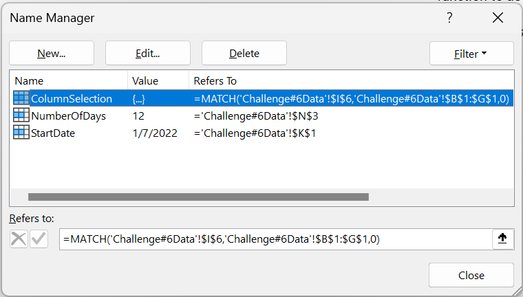
Thank you for participating in the Excel Challenge related to Name Manager, Data Validation and Indirect Function! I hope you found this challenge to be a fun and engaging way to improve your Excel skills and learn more about how to perform conditional summation in Excel.

Here is my solution to Workout #6:

=SUM(OFFSET(A1, MATCH(K1,A2:A366,0),MATCH(I6,B1:G1,0),(K3-K1)+1))

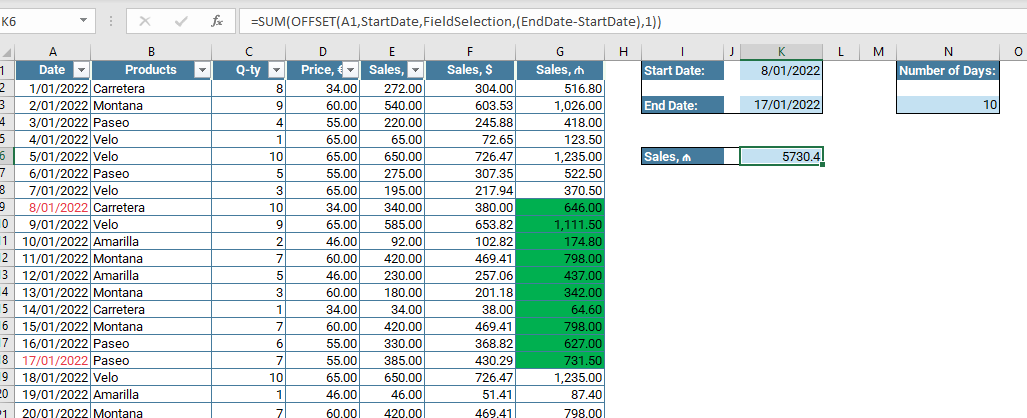
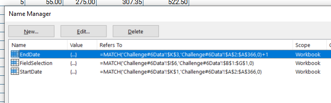
This formula calculates the sum of a selected field (I6) by using the OFFSET function to determine the range. The starting point for the range is cell A1, and the rows are determined by finding the start date (K1) in the A2:A366 range using the MATCH function. The columns are determined by finding the field name (I6) in the header row of the table (B1:G1) using MATCH. The height of the range is determined by subtracting the start date (K1) from the end date (K3) and adding 1.

Challenge #6 with Solution.xlsx (8.3 MB)

Once again, thank you for participating in this Excel Challenge, and I look forward to seeing you in future challenges and learning opportunities!

Keith · May 13, 2023, 10:34pm

Hi @IlgarZarbaliyev,

Trying to catch up on pass workouts.

Here is the solution to the problem

=SUM(OFFSET(A1, MATCH(K1,A2:A366,0),MATCH(I6,B1:G1,0),(K3-K1)+1))

file is attached
Excel Workout Challenge #6 Keith Smith.xlsx (8.3 MB)

thanks
Keith

Sujan_Chhetri · August 3, 2023, 7:38pm

@IlgarZarbaliyev - I never knew about the OFFSET() function, a new learning for me. Thanks for sharing this workout.

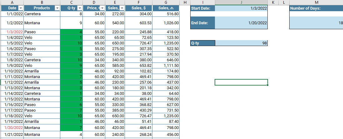
Please find my approach below:

I have revised the “Number of Days” calculation to incorporate a logical condition, ensuring that the Start Date is not greater than the End Date: =IF($J$1<=$J$3, $J$3-$J$1+1, “Start Date Cannot be greater than End Date”)
Formula for calculation total Quantity based on dynamic range selection: =IFERROR(SUM(OFFSET($A$2,MATCH($J$1,Dates,0)-1,2,$M$3,1)),“Check the Start and End Date”)

Here’s my workout: Challenge #6.xlsx (8.3 MB)

IlgarZarbaliyev · August 3, 2023, 8:21pm

Awesome!