INDEX is a function in Excel that is used to retrieve a value or a reference to a cell from a specific row and column within a range of cells or an array.
Match Function
MATCH is a function in Excel that is used to search for a value in a range of cells and return its position or index number within that range.
Goals
Please follow the directions given below, which include downloading the Excel worksheet required to perform the challenge tasks. Once you have completed the download, proceed to take the challenge and test your skills.
Task
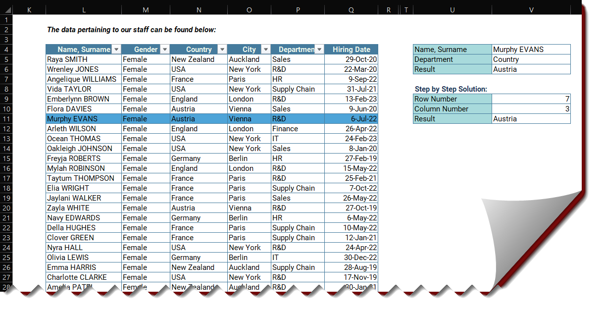
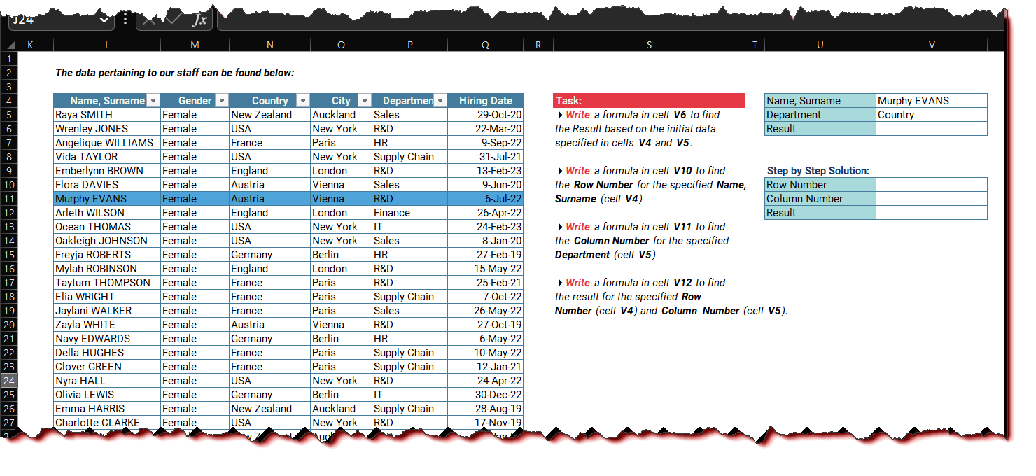
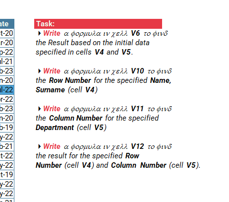
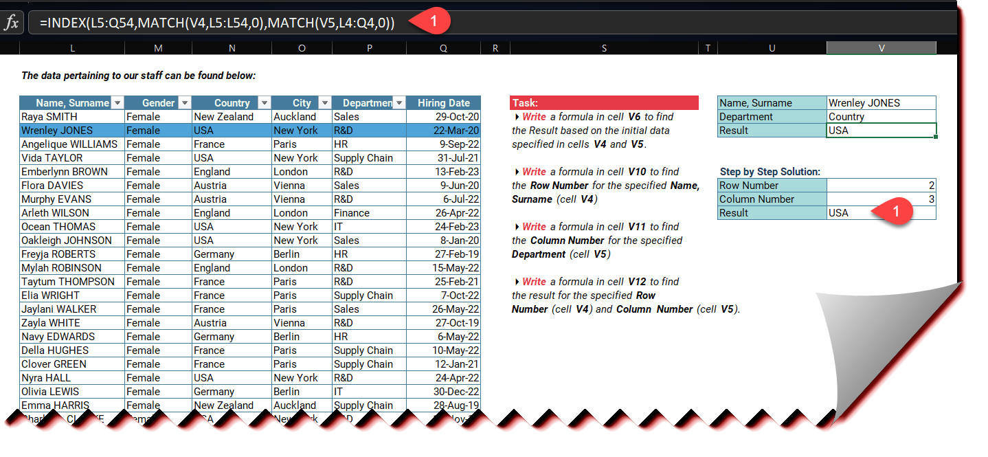
Write a formula in cell V6 to find the Result based on the initial data specified in cells V4 and V5.
Write a formula in cell V10 to find the Row Number for the specified Name, Surname (cell V4)
Write a formula in cell V11 to find the Column Number for the specified
Department (cell V5)
Write a formula in cell V12 to find the result for the specified Row
Number (cell V4) and Column Number (cell V5).
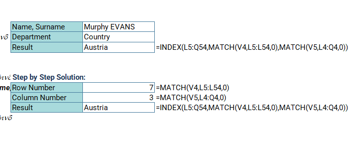
Two way lookup Solution Formula with Index - Match
Result =INDEX($L$5:$Q$54,MATCH(V4,$L$5:$L$54,0),MATCH(V5,$L$4:$Q$4,0))
Step By Step Solution
Row number =MATCH(V4,L5:L54,0)
Column=MATCH(V5,L4:Q4,0)
This can also be achieved by other lookup functions like XLOOKUP. But I will stick to INDEX and Match. Making the data range absolute is also not necessary. With XMATCH the third argument is not necessary as it will be approximate match by default.
I’ve only used Index & Match at an Excel Formulas and Functions course and once at work to make a Matrix for the factories.
Hover over the functions in Excel:
MATCH Returns the relative position of an item in an array that matches a specified value in a specified order
XMATCH Returns the relative position of an item in an array. By default, exact match is required
Why can’t MATCH just say: Returns the relative position of an item in an array?
In short, save a comma and a zero for each MATCH. Challenge #4.xlsx (8.3 MB)
Thank you for participating in the Excel Challenge related to Index & Match Functions! I hope you found this challenge to be a fun and engaging way to improve your Excel skills and learn more about how to perform conditional summation in Excel.
We use the Index and Match functions to search for values at Column and Row intersections. Index function finds the value at the intersection of row and column numbers shown in the specified array. We can find the Row and Column numbers with the Match function.
The formulas to write cells V6, V10, V11 and V12 are as follows, respectively: