— CAN YOU SOLVE THIS - EXCEL CHALLENGE 18 —
(Power Query solutions also welcome for Excel Challenges)
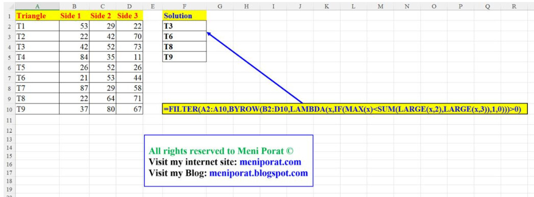
Provide a formula to list all Triangles from A2:A10. Given 3 sides, something is a Triangle if sum of two sides is > third side. Hence, for sides a, b, c, it is a Triangle if all 3 are met - a+b>c, b+c>a, c+a>b.
(Post answers in Comment. Your formula need not be different from others as long as you have worked out your formula independently)
Download Practice File - https://lnkd.in/dp-HK3HW
#excel, #advancedexcel, #excelchallenge, #excelproblem, #excelquestion, #excelsolution, #excelformulas, #excelfunctions, #exceltips, #exceltricks, #powerquerychallenge, #powerbichallenge, #powerqueryproblem, #M, #powerpivot
Excel BI’s LinkedIn Post
1 Like
Formula for Identifying Triangles
Quadri Atharu Triangle or not- SOlution.xlsx (392.6 KB)
=LET(a,B2:B10,b,C2:C10,c,D2:D10,
(FILTER(A2:A10,((a+b)>c)*((b+c)>a)*((c+a)>b))))
Here is one way to do it in Excel.
=FILTER(A2:A10, BYROW(B2:D10, LAMBDA(a, SUM(SMALL(a, {1, 2})) > MAX(a))))
Triangle or not.xlsx (17.8 KB)
I finished with almost the same formula as Sergei Baklan so, to vary the story, I used Heron’s formula for the area
A² = s(s-a)(s-b)(s-c)
giving
= FILTER(triangle,
BYROW(sides, LAMBDA(d, LET(
s, SUM(d)/2,
A², PRODUCT(s, s-d),
A²>0 )))
)
Who cares about short when there is fun to be had!
I have used the logic to iterate 3 sides and at each side check if the current value is less than the sum of all the other sides excluding current side.
let
  Source = DataSource,
  AddedCustom = Table.AddColumn (
    Source,
    "Custom",
    (CurrentRow) =>
      let
        TriangleValues =
          Record.ToList (
            Record.RemoveFields ( CurrentRow, "Triangle" )
          ),
        Result =
          List.AllTrue (
            List.Transform (
              TriangleValues,
              (CurrentValue) =>
                CurrentValue
                  < List.Sum (
                    List.RemoveItems ( TriangleValues, { CurrentValue } )
                  )
            )
          )
      in
        Result,
        Logical.Type
  ),
  FilteredRows = Table.SelectRows ( AddedCustom, each ([Custom] = true ) )
in
  FilteredRows
=INDEX(FILTER(A2:D10,(B2:B10+C2:C10>D2:D10)*(C2:C10+D2:D10>B2:B10)*(D2:D10+B2:B10>C2:C10)),,1)
Excel BI I have removed INDEX. Its not even needed if I just reference A2:A10 instead of A2:D10
=FILTER(A2:A10,(B2:B10+C2:C10>D2:D10)*(C2:C10+D2:D10>B2:B10)*(D2:D10+B2:B10>C2:C10))
Can’t verify, but this is my submission,
=FILTER(TAKE(Rng,,1), BYROW(DROP(Rng,,1), LAMBDA(x, MEDIAN(x) > MAX(x) - MIN(x))))
Selecting a single column just irritates me.
= FILTER(
    CHOOSECOLS(data, 1),
    BYROW(
      CHOOSECOLS(data, 2, 3, 4),
      LAMBDA(a, SUM(SMALL(a, {1,2})) > MAX(a))))
Here is an unconventional power query one.
let
  Source = Excel.CurrentWorkbook(){[ Name = "data" ]}[Content],
  Calc = Table.AddColumn (
    Source,
    "Calc",
    ( f ) =>
      let
        a = Record.ToList ( f ),
        b = List.Sort ( List.Skip ( a ) ),
        d = List.Sum ( List.FirstN ( b, 2 ) ) > List.Sum ( { List.Last ( b ) } )
      in
        d
  ),
  Result = Table.SelectRows ( Calc, each ( [Calc] = true ) )[[Triangle]]
in
  Result
My Power Query solution:
let
  Source = Table.TransformColumnTypes(#"Triangles Raw",{{"Side 1", Int64.Type}, {"Side 2", Int64.Type}, {"Side 3", Int64.Type}}),
  TestSides = Table.AddColumn(Source, "Custom", each
    if [Side 1] + [Side 2] <= [Side 3] then 0 else
    if [Side 1] + [Side 3] <= [Side 2] then 0 else
    if [Side 2] + [Side 3] <= [Side 1] then 0 else
    1),
  Cleanup = Table.RenameColumns( Table.RemoveColumns( Table.SelectRows(TestSides, each ([Custom] = 1)), {"Side 1", "Side 2", "Side 3", "Custom"}), {"Triangle", "Expected Answer"})
in
  Cleanup
=FILTER(

A2:A10,

(B2:B10+C2:C10>D2:D10)*
(C2:C10+D2:D10>B2:B10)*
(B2:B10+D2:D10>C2:C10)

)
Power Query variation
let
  Source = Excel.CurrentWorkbook(){[Name="data"]}[Content],
  #"Promoted Headers" = Table.PromoteHeaders(Source, [PromoteAllScalars=true]),

  Triangle =
    Table.SelectColumns(
      Table.SelectRows( #"Promoted Headers",
        (_) => [ a= List.LastN( Record.FieldValues(_), 3),
             b=List.Max(a)/List.Sum(a) < 0.5 ][b] ),
        Table.ColumnNames(#"Promoted Headers"){0} )
in
  Triangle
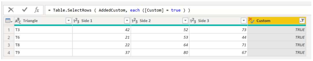
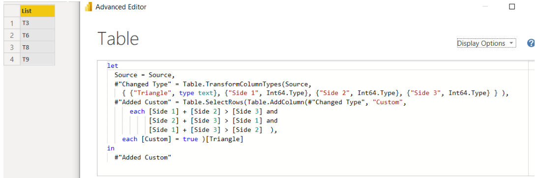
Excel BI - Power Query Solution
let
Source = Source,
#"Changed Type" = Table.TransformColumnTypes(Source,
{ {"Triangle", type text}, {"Side 1", Int64.Type}, {"Side 2", Int64.Type}, {"Side 3", Int64.Type} } ),
#"Added Custom" = Table.SelectRows(Table.AddColumn(#"Changed Type", "Custom",
each [Side 1] + [Side 2] > [Side 3] and
[Side 2] + [Side 3] > [Side 1] and
[Side 1] + [Side 3] > [Side 2] ),
each [Custom] = true )[Triangle]
in
#"Added Custom"
let
 Fonte = Excel.CurrentWorkbook(){[Name="Tabela1"]}[Content],
 cond = Table.SelectRows(
 Table.AddColumn(Fonte, "Result", each

 if [Side 1] + [Side 2] > [Side 3] and
 [Side 2] + [Side 3] > [Side 1] and
 [Side 3] + [Side 1] > [Side 2] then true else false),

 each [Result] = true ) [[Triangle]]
in
 cond
Power BI - M Code
#"Changed Type1" = Table.TransformColumnTypes(#"Promoted Headers",{{"Triangle", type text}, {"Side 1", Int64.Type}, {"Side 2", Int64.Type}, {"Side 3", Int64.Type}}),
 #"Added Custom" = Table.AddColumn(#"Changed Type1", "Custom", each if ([Side 1]+[Side 2] > [Side 3])
and ([Side 2]+[Side 3] > [Side 1])
and ([Side 1]+[Side 3] > [Side 2]) then 1
else 0),
 #"Filtered Rows" = Table.SelectRows(#"Added Custom", each ([Custom] = 1))
in
 #"Filtered Rows"
I am pretty sure this works correctly…
=FILTER(A2:A10,BYROW(B2:D10,LAMBDA(x,2*MAX(x)<SUM(x))))
As variant
=FILTER( A2:A10, BYROW(B2:D10, LAMBDA(v, MAX(v/SUM(v) ) < 0.5 ) ) )
I promise to rethink my solution and reduce the formula size.
=FILTER(A2:A10,((B2:B10+C2:C10>D2:D10)*(C2:C10+D2:D10>B2:B10)*(D2:D10+B2:B10>C2:C10))*ROW(A2:A10)>0)
The first formula without the FILTER function:
=LET(
a,B2:B10,
b,C2:C10,
c,D2:D10,
d,A2:A10,

TEXTSPLIT(
 TEXTJOIN(
 "-",
 ,
 IF(
 (a+b>c)*(b+c>a)*(a+c>b),
 d,
 ""
 )
 ),
 ,
 "-"
 )

)