— CAN YOU SOLVE THIS - EXCEL CHALLENGE 5 —
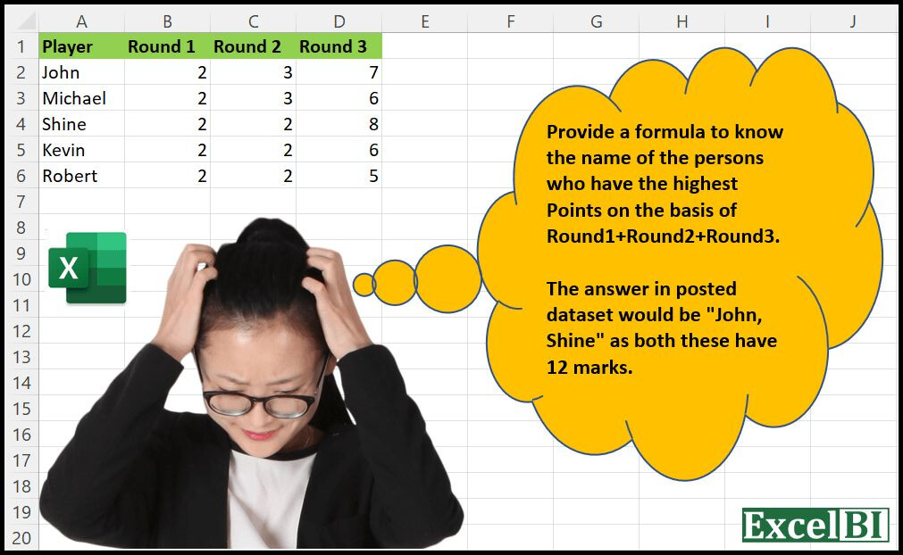
Provide a formula to know the name of the persons who have the highest Points on the basis of Round1+Round2+Round3.
(Post answers in Comment. Your formula need not be different from others as long as you have worked out your formula independently)
Download Practice File - https://lnkd.in/gTexCJBk
#excel , #advancedexcel , #excelchallenge , #excelproblem , #excelquestion , #excelsolution , #excelformulas , #excelfunctions , #exceltips , #exceltricks
Excel BI’s LinkedIn Post:
Quadri - Highest Points Solution.xlsx (953.2 KB)
Formula Used
=LET(x,BYROW(B2:D6,LAMBDA(x,SUM(x))),TEXTJOIN(", ",FILTER(A2:A6,x=MAX(x))))
=LET(x,BYROW(B2:D6,LAMBDA(x,SUM(x))),ARRAYTOTEXT(FILTER(A2:A6,x=MAX(x))))
Just for my own learning, here’s an OfficeScript / TypeScript approach.
function main(wb: ExcelScript.Workbook) {
  const rng: ExcelScript.Range = wb.getFirstWorksheet().getRangeByIndexes(1, 0, 5, 4);
  const newArr: (string | boolean | number)[][] = rng.getValues().map(x => [x[0], x.slice(1, 4).reduce((a, b) => Number(a) + Number(b), 0)]);
  const numArr: (number)[] = newArr.map(x => Number(x[1]));
  const max: number = numArr.sort((a: number, b: number) => a - b).reverse()[0]
  const result: string = newArr.filter((v) => v[1] === max).map(x => x[0]).join()
  console.log(result)
}
1 Like
Here is one way to do it in Excel.
=LET(
    _p, A2:A6,
    _sc, B2:D6,
    _tsc, MMULT(_sc, TOCOL(COLUMN(_sc) ^ 0)),
    _max, MAX(_tsc),
    _r, ARRAYTOTEXT(FILTER(_p, _tsc = _max)),
    _r
)
Here:
Highest Points.xlsx (17.5 KB)
Here is one way out with Power Query.
let
	Source   = Excel.CurrentWorkbook(){[ Name = "data" ]}[Content],
	Total    = Table.AddColumn (
		Source,
		"Total",
		each List.Sum ( List.Skip ( Record.FieldValues ( _ ) ) )
	),
	Max      = List.Max ( Total[Total] ),
	Filtered = Table.SelectRows ( Total, each ( [Total] = Max ) )[Player],
	Final    = Text.Combine ( Filtered, ", " )
in
	Final
Highest Points.xlsx (23.0 KB)
LinkedIn Post by: Tolga Demirci
w/ an applied E column;
=TEXTJOIN(",";;IF(MAXIFS($E$2:E2;$E$2:E2;FILTER(E2:E6;MAX(E2:E6);""))=MAX(E2:E6);A2:A6;""))
Sheet1 (2)
Player,Round 1,Round 2,Round 3,Round1+Round2+Round3
John,2,3,7,12,,
Michael,2,3,6,11,
Shine,2,2,8,12,
Kevin,2,2,6,10,
Robert,2,2,5,9,
LinkedIn Post by: Jardiel Euflázio
=TEXTJOIN
(
", ";;
IF(

SUBTOTAL(9;OFFSET(B1:D1;ROW(INDIRECT("1:"&ROWS(A2:A6)));))=
MAX(SUBTOTAL(9;OFFSET(B1:D1;ROW(INDIRECT("1:"&ROWS(A2:A6)));)));
A2:A6;
""

)
)
Love the SUBTOTAL function.
LinkedIn Post by: Bhavya Gupta
Solution Using Power Query -
let
Source = Excel.CurrentWorkbook(){[Name="Table1"]}[Content],
#"Unpivoted Other Columns" = Table.UnpivotOtherColumns(Source, {"Player"}, "Attribute", "Value"),
#"Grouped Rows" = [Table.Group](http://table.group/)(#"Unpivoted Other Columns", {"Player"}, {{"Total", each List.Sum([Value]), type number}}),
#"Filtered Rows" = Text.Combine( Table.SelectRows(#"Grouped Rows", each ([Total] = List.Max(#"Grouped Rows"[Total])))[Player],", ")
in
#"Filtered Rows"
LinkedIn ost by:محمد حلمي
=TEXTJOIN(" ";;IF(MMULT(B2:D6;{1;1;1})=
MAX(MMULT(B2:D6;{1;1;1}));A2:A6;""))
or
=LET(D;MMULT(B2:D6;{1;1;1});
TEXTJOIN(" ";;IF(D=MAX(D);A2:A6;"")))
LinkedIn Post by:Udit Kumar Chatterjee
Here is my solution in #PowerQuery :
let
Source = #"Challenge-05",

// get total points by players
unpivotRoundCols = Table.UnpivotOtherColumns(Source, {"Player"}, "Attribute", "Value"),
getTotalPoints = [Table.Group](http://table.group/)(
unpivotRoundCols, {"Player"}, {{"Total Points", each List.Sum([Value]), type number}}
),

// get highest point
maxPoints = List.Max(Table.Column(getTotalPoints, "Total Points")),

// filter table by highest points
filteredTable = Table.SelectRows(getTotalPoints, each [Total Points] = maxPoints),
getPlayerNames = Table.Column(filteredTable, "Player")
in
getPlayerNames
LinkedIn Post by:Aditya Kumar Darak
It is one way to do in Power Query.
let
  Source = Excel.CurrentWorkbook(){[ Name = "data" ]}[Content],
  Total = Table.AddColumn (
    Source,
    "Total",
    each List.Sum ( { [Round 1], [Round 2], [Round 3] } )
  ),
  Max = List.Max ( Total[Total] ),
  Filtered = Table.SelectRows ( Total, each ( [Total] = Max ) )[Player],
  Final = Text.Combine ( Filtered, ", " )
in
  Final
LinkedIn Post by: Bhavya Gupta
=LET(a, BYROW(B2:D6,LAMBDA(x, SUM(x))),TEXTJOIN(", ",FALSE,FILTER(A2:A6,a=MAX(a))))
LinkedIn Post by:Muthukumar Rasu
=TEXTJOIN(",",TRUE,IF(E1:E5=MAX(E1:E5),A1:A5,""))
I applied sum formula in E Column for each row
LinkedIn Post by:Sergei Baklan
If with DAX to return as PivotTable
---
Top Players :=
VAR addSum =
  ADDCOLUMNS ( data, "Total", data[Round 1] + data[Round 2] + data[Round 3] )
VAR maxPoint =
  MAXX ( addSum, [Total] )
VAR names =
  CONCATENATEX ( FILTER ( addSum, [Total] = maxPoint ), data[Player], ", " )
RETURN
  names
LinkedIn Post by: Nabil Mourad
=ARRAYTOTEXT(
  LET(
  a,BYROW(B2:D6,LAMBDA(x,SUM(x))),
  b,A2:A6,
  FILTER(b,a=MAX(a))
   )
)
LinkedIn Post by:Hugo Barreto
=UNIRCADENAS(";";;SI((B2:B6)+(C2:C6)+(D2:D6)=MAX((B2:B6)+(C2:C6)+(D2:D6));A2:A6;""))
LinkedIn Post by:Rick Rothstein
As long as you do not have a lot of rounds to process, this would work…=LET(S,B2:B6+C2:C6+D2:D6,TEXTJOIN(", ",1,IF(S=MAX(S),A2:A6,"")))
LinkedIn Post by:Juliano Santos Lima
=FILTER(A2:A6,E2:E6=MAX(MMULT(B2:D6,{1,1,1})))